Risk and Money Management In Algorithmic Trading

This chapter is concerned with managing risk as applied to quantitative trading strategies. This usually comes in two flavours, firstly identifying and mitigating internal and external factors that can affect the performance or operation of an algorithmic trading strategy and secondly, how to optimally manage the strategy portfolio in order to maximise growth rate and minimise account drawdowns.

In the first section we will consider different sources of risk (both intrinsic and extrinsic) that might affect the long-term performance of an algorithmic trading business – either retail or institutional.

In the second section we will look at money management techniques that can simultaneously protect our portfolio from ruin and also attempt to maximise the long-term growth rate of equity.

In the final section we consider institutional-level risk management techniques that can easily be applied in a retail setting to help protect trading capital.

1.) Sources of Risk

The are numerous sources of risk that can have an impact on the correct functioning of an algorithmic trading strategy. “Risk” is usually defined in this context to mean chance of account losses. However, I am going to define it in a much broader context to mean any factor that provides a degree of uncertainty and could affect the performance of our strategies or portfolio.

The broad areas of risk that we will consider include Strategy Risk, Portfolio Risk, Market Risk, Counterparty Risk and Operational Risk.

1.1] Strategy Risk:

Strategy risk, or model risk, encompasses the class of risks that arise from the design and implementation of a trading strategy based on a statistical model. It includes all of the previous issues we have discussed in the Successful Backtesting chapter, such as curve-fitting, survivorship bias and look-ahead bias. It also includes other topics related directly to the statistical analysis of the strategy model.

Any statistical model is based on assumptions. These assumptions are sometimes not considered in proper depth or ignored entirely. This means that the statistical model based upon these assumptions may be inappropriate and hence lead to poor predictive or inferential capability. A general example occurs in the setting of linear regression. Linear regression makes the assumption that the response data are homoscedastic (i.e. the responses have a constant variance in their errors). If this is not the case then linear regression provides less precision in the estimates of parameters.

Many quantitative strategies make use of descriptive statistics of historical price data. In particular, they will often use moments of the data such as the mean, variance, skew and kurtosis of strategy returns. Such models (including the Kelly Criterion outlined below) generally rely on these moments being constant in time. Under a market regime change these moments can be drastically altered and hence lead to degradation of the model. Models with “rolling parameters” are usually utilised in order to mitigate this issue.

1.2] Portfolio Risk:

A Portfolio contains one or more strategies. Thus it is indirectly subject to Strategy Risk as outlined above. In addition there are specific risks that occur at the portfolio level. These are usually only considered in an institutional setting or in a high-end retail setting where portfolio tracking is being carried out on a stable of trading strategies.

When regressing portfolio returns to a set of factors, such as industry sectors, asset classes or groups of financial entities it is possible to ascertain if the portfolio is heavily “loaded” into a particular factor. For instance, an equities portfolio may be extremely heavy on technology stocks and thus is extremely exposed to any issues that affect the tech sector as a whole. Hence it is often necessary – at the portfolio level – to override particular strategies in order to account for overloaded factor risk. This is often a more significant concern in an institutional setting where there is more capital to be allocated and the preservation of capital takes precedence to the long-term growth rate of the capital. However, it should certainly be considered even as a retail algorithmic trading investor.

Another issue that is largely an institutional issue (unless trading more illiquid assets) are limits on daily trading volume. For retail traders, executing strategies in the large-cap or commodities futures markets, there is no real concern regarding market impact. However, in less liquid instruments one has to be careful to not be trading a significant percentage of the daily traded volume, due to potential market impact and thus invalidation of a previously backtested trading model (which often do not take into account market impact). To avoid this it is necessary to calculate the average daily volume (using a mean over a loopback period, for instance) and stay within small percentage limits of this figure.

Running a portfolio of strategies brings up the issue of strategy correlation. Correlations can be estimated via statistical techniques such as the Pearson Product Moment Correlation Coefficient. However, correlation itself is not a static entity and is also subject to swift change, especially under market-wide liquidity constraints, often known as financial contagion. In general, strategies should be designed to avoid correlation with each other by virtue of differing asset classes or time horizons. Rolling correlations can be estimated over a large time-period and should be a standard part of your backtest, if considering a portfolio approach.

1.3] Counterparty Risk:

Counterparty risk is generally considered a form of credit risk. It is the risk that a counterpart will not pay an obligation on a financial asset under which they are liable. There is an entire subset of quantitative finance related to the pricing of counterpart risk hedging instruments, but this is not of primary interest to us as retail algorithmic traders. We are more concerned with the risk of default from suppliers such as an exchange or brokerage.

While this may seem academic, I can personally assure you that these issues are quite real! In an institutional setting I have experienced first hand a brokerage bankruptcy under conditions that meant not all of the trading capital was returned. Thus I now factor such risks into a portfolio. The suggested means of mitigating this issue is to utilise multiple brokerages, although when trading under margin this can make the trading logistics somewhat tricky.

Counterparty risk is generally more of a concern in an institutional setting so I won’t dwell on it too much here!

1.4] Operational Risk:

Operation risk encompasses sources of risk from within a fund or trading operational infrastructure, including business/entrepreneurial risk, IT risk and external regulatory or legal changes. These topics aren’t often discussed in any great depth, which I believe is somewhat short-sighted since they have the potential to completely halt a trading operation permanently.

Infrastructure risk is often associated with information technology systems and other related trading infrastructure. This also includes employee risk (such as fraud, sudden departure). As the scale of an infrastructure grows so does the likelihood of the “single point of failure” (SPOF). This is a critical component in the trading infrastructure that, under malfunction, can lead to a catastrophe halting of the entire operation. In the IT sense, this is usually the consequence of a badly thought out architecture. In a non-IT sense this can be the consequence of a badly designed organisation chart.

These issues are still entirely relevant for the retail trader. Often, an IT/trading infrastructure can end up being “patchy” and “hacked together”. In addition, poor record keeping and other administrative failures can lead to huge potential tax burdens. Thankfully, “cloud” architecture provides the ability for redundancy in systems and automation of processes can lead to solid administrative habits. This type of behaviour, that is consideration of risks from sources other than the market and the strategy, can often make the difference between a successful long-term algorithmic trader and the individual who gives up due to catastrophic operation breakdown.

An issue that affects the hedge fund world is that of reporting and compliance. Post-2008 legislation has put a heavy burden on asset management firms, which can have a large impact on their cash-flow and operating expenditure. For an individual thinking of incorporating such a firm, in order to expand a strategy or run with external funds, it is prudent to keep on top of the legislation and regulatory environment, since it is somewhat of a “moving target”.

2.) Money Management

This section deals with one of the most fundamental concepts in trading – both discretionary and algorithmic – namely, money management. A naive investor/trader might believe that the only important investment objective is to simply make as much money as possible. However the reality of long-term trading is more complex. Since market participants have differing risk preferences and constraints there are many objectives that investors may possess.

Many retail traders consider the only goal to be a continual increase of account equity, with little or no consideration given to the “risk” of a strategy that achieves this growth. More sophisticated retail investors measure account drawdowns, and depending upon their risk preferences, may be able to cope with a substantial drop in account equity (say 50%). The reason they can deal with a drawdown of this magnitude is that they realise, quantitatively, that this behaviour may be optimal for the long-term growth rate of the portfolio, via the use of leverage.

An institutional investor is likely to consider risk in a different light. Often institutional investors have mandated maximum drawdowns (say 20%), with significant consideration given to sector allocation and average daily volume limits. They would be additional constraints on the “optimisation problem” of capital allocation to strategies. These factors might even be more important than maximising the long-term growth rate of the portfolio.

Thus we are in a situation where we can strike a balance between maximising long-term growth rate via leverage and minimising our “risk” by trying to limit the duration and extent of the drawdown. The major tool that will help us achieve this is called the Kelly Criterion.

2.1] Kelly Criterion:

Within this section the Kelly Criterion is going to be our tool to control leverage of, and allocation towards, a set of algorithmic trading strategies that make up a multi-strategy portfolio.

We will define leverage as the ratio of the size of a portfolio to the actual account equity within that portfolio. To make this clear we can use the analogy of purchasing a house with a mortgage. Your down payment (or “deposit” for those of us in the UK!) constitutes your account equity, while the down payment plus the mortgage value constitutes the equivalent of the size of a portfolio. Thus a down payment of 50,000 USD on a 200,000 USD house (with a mortgage of 150,000 USD) constitutes a leverage of (150000 + 50000)/50000 = 4. Thus in this instance you would be 4x leveraged on the house. A margin account portfolio behaves similarly. There is a “cash” component and then more stock can be borrowed on margin, to provide the leverage.

Before we state the Kelly Criterion specifically I want to outline the assumptions that go into its derivation, which have varying degrees of accuracy:

Each algorithmic trading strategy will be assumed to possess a returns stream that is normally distributed (i.e. Gaussian). Further, each strategy has its own fixed mean and standard deviation of returns. The formula assumes that these mean and std values do not change, i.e. that they are same in the past as in the future. This is clearly not the case with most strategies, so be aware of this assumption.
The returns being considered here are excess returns, which means they are net of all financing costs such as interest paid on margin and transaction costs. If the strategy is being carried out in an institutional setting, this also means that the returns are net of management and performance fees.
All of the trading profits are reinvested and no withdrawals of equity are carried out. This is clearly not as applicable in an institutional setting where the above mentioned management fees are taken out and investors often make withdrawals.
All of the strategies are statistically independent (there is no correlation between strategies) and thus the covariance matrix between strategy returns is diagonal.

Now we come to the actual Kelly Criterion! Let’s imagine that we have a set of N algorithmic trading strategies and we wish to determine both how to apply optimal leverage per strategy in order to maximise growth rate (but minimise drawdowns) and how to allocate capital between each strategy. If we denote the allocation between each strategy i as a vector f of length N, s.t.

= (f₁,…,f_N), then the Kelly Criterion for optimal allocation to each strategy f_iis given by:

f_i= µ_i/σ_i²

Where µ_iare the mean excess returns and σ_iare the standard deviation of excess returns for a strategy i. This formula essentially describes the optimal leverage that should be applied to each strategy.

While the Kelly Criterion f_igives us the optimal leverage and strategy allocation, we still need to actually calculate our expected long-term compounded growth rate of the portfolio, which we denote by g. The formula for this is given by:

g = r + S²/2

Where r is the risk-free interest rate, which is the rate at which you can borrow from the broker, and S is the annualised Sharpe Ratio of the strategy. The latter is calculated via the annualised mean excess returns divided by the annualised standard deviations of excess returns. See the previous chapter on Performance Measurement for details on the Sharpe Ratio.

A Realistic Example

Let’s consider an example in the single strategy case (i = 1). Suppose we go long a mythical stock XYZ that has a mean annual return of m = 10.7% and an annual standard deviation of σ = 12.4%. In addition suppose we are able to borrow at a risk-free interest rate of r = 3.0%. This implies that the mean excess returns are µ = m − r = 10.7 − 3.0 = 7.7%. This gives us a Sharpe Ratio of S = 0.077/0.124 = 0.62.

With this we can calculate the optimal Kelly leverage via f = µ/σ²= 0.077/0.124²= 5.01. Thus the Kelly leverage says that for a 100,000 USD portfolio we should borrow an additional 401,000 USD to have a total portfolio value of 501,000 USD. In practice it is unlikely that our brokerage would let us trade with such substantial margin and so the Kelly Criterion would need to be adjusted.

We can then use the Sharpe ratio S and the interest rate r to calculate g, the expected long-term compounded growth rate. g = r + S²/2 = 0.03 + 0.62²/2 = 0.22, i.e. 22%. Thus we should expect a return of 22% a year from this strategy.

Kelly Criterion in Practice

It is important to be aware that the Kelly Criterion requires a continuous rebalancing of capital allocation in order to remain valid. Clearly this is not possible in the discrete setting of actual trading and so an approximation must be made. The standard “rule of thumb” here is to update the Kelly allocation once a day. Further, the Kelly Criterion itself should be recalculated periodically, using a trailing mean and standard deviation with a lookback window. Again, for a strategy that trades roughly once a day, this lookback should be set to be on the order of 3-6 months of daily returns.

Here is an example of rebalancing a portfolio under the Kelly Criterion, which can lead to some counter-intuitive behaviour. Let’s suppose we have the strategy described above. We have used the Kelly Criterion to borrow cash to size our portfolio to 501,000 USD. Let’s assume we make a healthy 5% return on the following day, which boosts our account size to 526,050 USD. The Kelly Criterion tells us that we should borrow more to keep the same leverage factor of 5.01. In particular our account equity is 126,050 USD on a portfolio of 526,050, which means that the current leverage factor is 4.17. To increase it to 5.01, we need to borrow an additional 105,460 USD in order to increase our account size to 631,510.5 USD (this is 5.01 × 126050).

Now consider that the following day we lose 10% on our portfolio (ouch!). This means that the total portfolio size is now 568,359.45 USD (631510.5 × 0.9). Our total account equity is now 62,898.95 USD (126050 − 631510.45 × 0.1). This means our current leverage factor is 568359.45/62898.95 = 9.03. Hence we need to reduce our account by selling 253,235.71 USD of stock in order to reduce our total portfolio value to 315,123.73 USD, such that we have a leverage of 5.01 again (315123.73/62898.95 = 5.01).

Hence we have bought into a profit and sold into a loss. This process of selling into a loss may be extremely emotionally difficult, but it is mathematically the “correct” thing to do, assuming that the assumptions of Kelly have been met! It is the approach to follow in order to maximise long-term compounded growth rate.

You may have noticed that the absolute values of money being re-allocated between days were rather severe. This is a consequence of both the artificial nature of the example and the extensive leverage employed. 10% loss in a day is not particularly common in higher-frequency algorithmic trading, but it does serve to show how extensive leverage can be on absolute terms. Since the estimation of means and standard deviations are always subject to uncertainty, in practice many traders tend to use a more conservative leverage regime such as the Kelly Criterion divided by two, affectionately known as “half-Kelly“. The Kelly Criterion should really be considered as an upper bound of leverage to use, rather than a direct specification. If this advice is not heeded then using the direct Kelly value can lead to ruin (i.e. account equity disappearing to zero) due to the non-Gaussian nature of the strategy returns.

Should You Use The Kelly Criterion?

Every algorithmic trader is different and the same is true of risk preferences. When choosing to employ a leverage strategy (of which the Kelly Criterion is one example) you should consider the risk mandates that you need to work under. In a retail environment you are able to set your own maximum drawdown limits and thus your leverage can be increased. In an institutional setting you will need to consider risk from a very different perspective and the leverage factor will be one component of a much larger framework, usually under many other constraints.

3.) Risk Management

3.1] Value-at-Risk:

Estimating the risk of loss to an algorithmic trading strategy, or portfolio of strategies, is of extreme importance for long-term capital growth. Many techniques for risk management have been developed for use in institutional settings. One technique in particular, known as Value at Risk or VaR, will be the topic of this section.

We will be applying the concept of VaR to a single strategy or a set of strategies in order to help us quantify risk in our trading portfolio. The definition of VaR is as follows:

VaR provides an estimate, under a given degree of confidence, of the size of a loss from a portfolio over a given time period.

In this instance “portfolio” can refer to a single strategy, a group of strategies, a trader’s book, a prop desk, a hedge fund or an entire investment bank. The “given degree of confidence” will be a value of, say, 95% or 99%. The “given time period” will be chosen to reflect one that would lead to a minimal market impact if a portfolio were to be liquidated.

For example, a VaR equal to 500,000 USD at 95% confidence level for a time period of a day would simply state that there is a 95% probability of losing no more than 500,000 USD in the following day. Mathematically this is stated as:

P(L ≤ −5.0 × 10⁵) = 0.05

Or, more generally, for loss L exceeding a value V aR with a confidence level c we have:

P(L ≤ −V aR) = 1 − c

The “standard” calculation of VaR makes the following assumptions:

Standard Market Conditions – VaR is not supposed to consider extreme events or “tail risk”, rather it is supposed to provide the expectation of a loss under normal “day-to-day” operation.
Volatilities and Correlations – VaR requires the volatilities of the assets under consideration, as well as their respective correlations. These two quantities are tricky to estimate and are subject to continual change.
Normality of Returns – VaR, in its standard form, assumes the returns of the asset or portfolio are normally distributed. This leads to more straightforward analytical calculation, but it is quite unrealistic for most assets.

4.) Advantages and Disadvantages

VaR is pervasive in the financial industry, hence you should be familiar with the benefits and drawbacks of the technique. Some of the advantages of VaR are as follows:

VaR is very straightforward to calculate for individual assets, algo strategies, quant portfolios, hedge funds or even bank prop desks.
The time period associated with the VaR can be modified for multiple trading strategies that have different time horizons.
Different values of VaR can be associated with different forms of risk, say broken down by asset class or instrument type. This makes it easy to interpret where the majority of portfolio risk may be clustered, for instance.
Individual strategies can be constrained as can entire portfolios based on their individual VaR.
VaR is straightforward to interpret by (potentially) non-technical external investors and fund managers.

However, VaR is not without its disadvantages:

VaR does not discuss the magnitude of the expected loss beyond the value of VaR, i.e. it will tell us that we are likely to see a loss exceeding a value, but not how much it exceeds it.
It does not take into account extreme events, but only typical market conditions.
Since it uses historical data (it is rearward-looking) it will not take into account future market regime shifts that can change volatilities and correlations of assets.

VaR should not be used in isolation. It should always be used with a suite of risk management techniques, such as diversification, optimal portfolio allocation and prudent use of leverage.

Methods of Calculation

As of yet we have not discussed the actual calculation of VaR, either in the general case or a concrete trading example. There are three techniques that will be of interest to us. The first is the variance-covariance method (using normality assumptions), the second is a Monte Carlo method (based on an underlying, potentially non-normal, distribution) and the third is known as historical bootstrapping, which makes use of historical returns information for assets under consideration.

In this section we will concentrate on the Variance-Covariance Method.

Variance-Covariance Method

Consider a portfolio of P dollars, with a confidence level c. We are considering daily returns, with asset (or strategy) historical standard deviation σ and mean µ. Then the daily VaR, under the variance-covariance method for a single asset (or strategy) is calculated as:

P − (P(α(1 − c) + 1))

Where α is the inverse of the cumulative distribution function of a normal distribution with mean µ and standard deviation σ.

We can use the SciPy and pandas libraries in order to calculate these values. If we set P = 10⁶and c = 0.99, we can use the SciPy ppf method to generate the values for the inverse cumulative distribution function to a normal distribution with µ and σ obtained from some real financial data, in this case the historical daily returns of CitiGroup (we could easily substitute the returns of an algorithmic strategy in here):

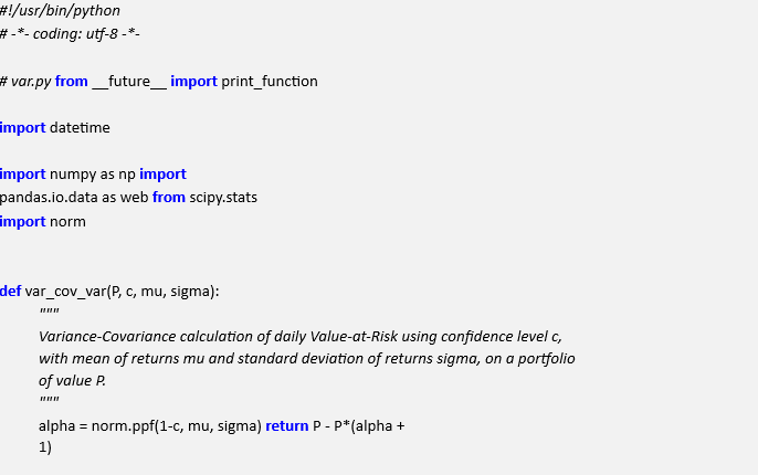
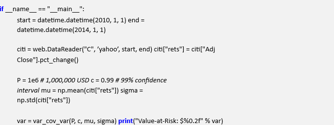
The calculated value of VaR is given by:

VaR is an extremely useful and pervasive technique in all areas of financial management, but it is not without its flaws. David Einhorn, the renowned hedge fund manager, has famously described VaR as “an airbag that works all the time, except when you have a car accident.” Indeed, you should always use VaR as an augmentation to your risk management overlay, not as a single indicator!