Performance Measurement In Algorithmic Trading

Performance measurement is an absolutely crucial component of algorithmic trading. Without assessment of performance, along with solid record keeping, it is difficult, if not impossible, to determine if our strategy returns have been due to luck or due to some actual edge over the market.

In order to be successful in algorithmic trading it is necessary to be aware of all of the factors that can affect the profitability of trades, and ultimately strategies. We should be constantly trying to find improvements in all aspects of the algorithmic trading stack. In particular we should always be trying to minimise our transaction costs (fees, commission and slippage), improve our software and hardware, improve the cleanliness of our data feeds and continually seek out new strategies to add to a portfolio. Performance measurement in all these areas provides a yardstick upon which to measure alternatives.

Ultimately, algorithmic trading is about generating profits. Hence it is imperative that we measure the performance, at multiple levels of granularity, of how and why our system is producing these profits. This motivates performance assessment at the level of trades, strategies and portfolios. In particular we are looking out for:

Whether the systematic rules codified by the strategy actually produce a consistent return and whether the strategy possesses positive performance in the backtests.
Whether a strategy maintains this positive performance in a live implementation or whether it needs to be retired.
The ability to compare multiple strategies/portfolios such that we can reduce the opportunity cost associated with allocating a limited amount of trading capital.

The particular items of quantitative analysis of performance that we will be interested in are as follows:

Returns – The most visible aspect of a trading strategy concerns the percentage gain since inception, either in a backtest or a live trading environment. The two major performance measures here are Total Return and Compound Annual Growth Rate (CAGR).
Drawdowns – A drawdown is a period of negative performance, as defined from a prior high-water mark, itself defined as the previous highest peak on a strategy or portfolio equity curve. We will define this more concretely below, but you can think of it for now as a (somewhat painful!) downward slope on your performance chart.
Risk – Risk comprises many areas, and we’ll spend significant time going over them in the following chapter, but generally it refers to both risk of capital loss, such as with drawdowns, and volatility of returns. The latter usually being calculated as an annualised standard deviation of returns.
Risk/Reward Ratio – Institutional investors are mainly interested with risk-adjusted returns. Since higher volatility can often lead to higher returns at the expense of greater drawdowns, they are always concerned with how much risk is being taken on per unit of return. Consequently a range of performance measures have been invented to quantify this aspect of strategy performance, namely the Sharpe Ratio, Sortino Ratio and CALMAR Ratio, among others. The out of sample Sharpe is often the first metric to be discussed by institutional investors when discussing strategy performance.
Trade Analysis – The previous measures of performance are all applicable to strategies and portfolios. It is also instructive to look at the performance of individual trades and many measures exist to characterise their performance. In particular, we will quantity the number of winning/losing trades, mean profit per trade and win/loss ratio among others.

Trades are the most granular aspect of an algorithmic strategy and hence we will begin by discussing trade analysis.

1.) Trade Analysis

The first step in analysing any strategy is to consider the performance of the actual trades. Such metrics can vary dramatically between strategies. A classic example would be the difference in performance metrics of a trend-following strategy when compared to a mean-reverting strategy.

Trend-following strategies usually consist of many losing trades, each with a likely small loss. The lesser quantity of profitable trades occur when a trend has been established and the performance from these positive trades can significantly exceed the losses of the larger quantity of losing trades. Pair-trading mean-reverting strategies display the opposing character. They generally consist of many small profitable trades. However, if a series does not mean revert in the manner expected then the long/short nature of the strategy can lead to substantial losses. This could potentially wipe out the large quantity of small gains.

It is essential to be aware of the nature of the trade profile of the strategy and your own psychological profile, as the two will need to be in alignment. Otherwise you will find that you may not be able to persevere through a period of tough drawdown.

We now review the statistics that are of interest to us as the trade level.

1.1] Summary Statistics:

When considering our trades, we are interested in the following set of statistics. Here “period” refers to the time period covered by the trading bar containing OHLCV data. For long-term strategies it is often the case that daily bars are used. For higher frequency strategies we may be interested in hourly or minutely bars.

Total Profit/Loss (PnL) – The total PnL straightforwardly states whether a particular trade has been profitable or not.
Average Period PnL – The avg. period PnL states whether a bar, on average, generates a profit or loss.
Maximum Period Profit – The largest bar-period profit made by this trade so far.
Maximum Period Loss – The largest bar-period loss made by this trade so far. Note that this says nothing about future maximum period loss! A future loss could be much larger than this.
Average Period Profit – The average over the trade lifetime of all profitable periods.
Average Period Loss – The average over the trade lifetime of all unprofitable periods.
Winning Periods – The count of all winning periods.
Losing Periods – The count of all losing periods.
Percentage Win/Loss Periods – The percentage of all winning periods to losing periods. Will differ markedly for trend-following and mean-reverting type strategies.

Thankfully, it is straightforward to generate this information from our portfolio output and so the need for manual record keeping is completely eliminated. However, this leads to the danger that we never actually stop to analyse the data!

It is imperative that trades are evaluated at least once or twice a month. Doing so is a useful early warning detection system that can help identify when strategy performance begins to degrade. It is often much better than simply considering the cumulative PnL alone.

2.) Strategy and Portfolio Analysis

Trade-level analysis is extremely useful in longer-term strategies, particularly with strategies that employ complex trades, such as those that involve derivatives. For higher-frequency strategies, we will be less interested in any individual trade and instead will want to consider the performance measures of the strategy instead. Obviously for longer-term strategies, we are equally as interested in the overall strategy performance. We are primarily interested in the following three key areas:

Returns Analysis – The returns of a strategy encapsulate the concept of profitability. In institutional settings they are generally quoted net of fees and so provide a true picture of how much money was made on money invested. Returns can be tricky to calculate, especially with cash inflows/outflows.
Risk/Reward Analysis – Generally the first consideration that external investors will have in a strategy is its out of sample Sharpe Ratio (which we describe below). This is an industry standard metric which attempts to characterise how much return was achieved per unit of risk.
Drawdown Analysis – In an institutional setting, this is probably the most important of the three aspects. The profile and extent of the drawdowns of a strategy, portfolio or fund form a key component in risk management. We’ll define drawdowns below.

Despite the fact that I have emphasised their institutional performance, as a retail trader these are still highly important metrics and with suitable risk management (see next chapter) will form the basis of a continual strategy evalation procedure.

2.1] Returns Analysis:

The most widely quoted figures when discussing strategy performance, in both institutional and retail settings, are often total return, annual returns and monthly returns. It is extremely common to see a hedge fund performance newsletter with a monthly return “grid”. In addition, everybody will want to know what the “return” of the strategy is.

Total return is relatively straightforward to calculate, at least in a retail setting with no external investors or cash inflows/outflows. In percentage terms it is simply calculated as:

r_t= (P_f− P_i)/P_i× 100

Where r_tis the total return, P_fis the final portfolio dollar value and P_iis the initial portfolio value. We are mostly interested in net total return, that is the value of the portfolio/fund after all trading/business costs have been deducted.

Note that this formula is only applicable to long-only un-leveraged portfolios. If we wish to add in short selling or leverage we need to modify how we calculate returns because we are technically trading on a larger borrowed portfolio than that used here. This is known as a margin portfolio.

For instance, consider the case where a trading strategy has gone long 1,000 USD of one asset and then shorted 1,000 USD of another asset. This is a dollar-neutral portfolio and the total notional traded is 2,000 USD. If 200 USD was generated from this strategy then gross return on this notional is 10%. It becomes more complex when you factor in borrowing costs and interest rates to fund the margin. Factoring in these costs leads to the net total return, which is the value that is often quoted as “total return”.

Equity Curve

The equity curve is often one of the most emphasised visualisations on a hedge fund performance report – assuming the fund is doing well! It is a plot of the portfolio value of the fund over time. In essence it is used to show how the account has grown since fund inception. Equally, in a retail setting it is used to show growth of account equity through time. See Fig 2.1 for a typical equity curve plot:

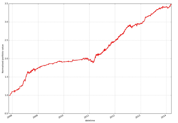
Figure 1: Typical intraday strategy equity curve

What is the benefit of such a plot? In essence it gives a “flavour” as to the past volatility of the strategy, as well as a visual indication of whether the strategy has suffered from prolonged periods of plateau or even drawdown. It essentially provides answers as to how the total return figure calculated at the end of the strategy trading period was arrived at.

In an equity curve we are seeking to determine how unusual historical events have shaped the strategy. For instance, a common question asks if there was excess volatility in the strategy around 2008. Another question might concern its consistency of returns.

One must be extremely careful with interpretation of equity curves as when marketed they are generally shown as “upward sloping lines”. Interesting insight can be gained via truncation of such curves, which can emphasise periods of intense volatility or prolonged drawdown that may otherwise not seem as severe when considering the whole time period. Thus an equity curve needs to be considered in context with other analysis, in particular risk/reward analysis and drawdown analysis.

2.2] Risk/Reward Analysis:

As we alluded to above the concept of risk-to-reward analysis is extremely important in an institutional setting. This does not mean that as a retail investor we can ignore the concept. You should pay significant attention to risk/reward metrics for your strategy as they will have a significant impact on your drawdowns, leverage and overall compound growth rate.

These concepts will be expanded on in the next chapter on Risk and Money Management. For now we will discuss the common ratios, and in particular the Sharpe Ratio, which is ubiquitous as a comparative measure in quantitative finance. Since it is held in such high regard across institutionalised quantitative trading, we will go into a reasonable amount of detail.

Sharpe Ratio

Consider the situation where we are presented with two strategies possessing identical returns. How do we know which one contains more risk? Further, what do we even mean by “more risk”? In finance, we are often concerned with volatility of returns and periods of drawdown. Thus if one of these strategies has a significantly higher volatility of returns we would likely find it less attractive, despite the fact that its historical returns might be similar if not identical. These problems of strategy comparison and risk assessment motivate the use of the Sharpe Ratio.

William Forsyth Sharpe is a Nobel-prize winning economist, who helped create the Capital Asset Pricing Model (CAPM) and developed the Sharpe Ratio in 1966 (later updated in 1994). The Sharpe Ratio S is defined by the following relation:

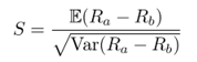
Where R_ais the period return of the asset or strategy and R_bis the period return of a suitable benchmark, such as a risk-free interest rate.

The ratio compares the mean average of the excess returns of the asset or strategy with the standard deviation of those excess returns. Thus a lower volatility of returns will lead to a greater Sharpe ratio, assuming identical mean returns.

The “Sharpe Ratio” often quoted by those carrying out trading strategies is the annualised Sharpe, the calculation of which depends upon the trading period of which the returns are measured. Assuming there are N trading periods in a year, the annualised Sharpe is calculated as follows:

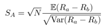
Note that the Sharpe ratio itself MUST be calculated based on the Sharpe of that particular time period type. For a strategy based on trading period of days, N = 252 (as there are 252 trading days in a year, not 365), and R_a, R_bmust be the daily returns. Similarly for hours N = 252×6.5 = 1638, not N = 252×24 = 6048, since there are only 6.5 hours in a trading day (at least for most US equities markets!).

The formula for the Sharpe ratio above alludes to the use of a benchmark. A benchmark is used as a “yardstick” or a “hurdle” that a particular strategy must overcome for it to worth consideration. For instance, a simple long-only strategy using US large-cap equities should hope to beat the S&P500 index on average, or match it for less volatility, otherwise what is to be gained by not simply investing in the index at far lower management/performance fees?

The choice of benchmark can sometimes be unclear. For instance, should a sector Exhange Traded Fund (ETF) be utilised as a performance benchmark for individual equities, or the S&P500 itself? Why not the Russell 3000? Equally should a hedge fund strategy be benchmarking itself against a market index or an index of other hedge funds?

There is also the complication of the “risk free rate”. Should domestic government bonds be used? A basket of international bonds? Short-term or long-term bills? A mixture? Clearly there are plenty of ways to choose a benchmark. The Sharpe ratio generally utilises the risk-free rate and often, for US equities strategies, this is based on 10-year government Treasury bills.

In one particular instance, for market-neutral strategies, there is a particular complication regarding whether to make use of the risk-free rate or zero as the benchmark. The market index itself should not be utilised as the strategy is, by design, market-neutral. The correct choice for a market-neutral portfolio is not to substract the risk-free rate because it is self-financing. Since you gain a credit interest, R_f, from holding a margin, the actual calculation for returns is: (R_a+ R_f) − R_f= R_a. Hence there is no actual subtraction of the risk-free rate for dollar neutral strategies.

Despite the prevalence of the Sharpe ratio within quantitative finance, it does suffer from some limitations. The Sharpe ratio is backward looking. It only accounts for historical returns distribution and volatility, not those occurring in the future. When making judgements based on the Sharpe ratio there is an implicit assumption that the past will be similar to the future.

This is evidently not always the case, particular under market regime changes.

The Sharpe ratio calculation assumes that the returns being used are normally distributed (i.e.

Gaussian). Unfortunately, markets often suffer from kurtosis above that of a normal distribution. Essentially the distribution of returns has “fatter tails” and thus extreme events are more likely to occur than a Gaussian distribution would lead us to believe. Hence, the Sharpe ratio is poor at characterising tail risk.

This can be clearly seen in strategies which are highly prone to such risks. For instance, the sale of call options aka “pennies under a steam roller”. A steady stream of option premia are generated by the sale of call options over time, leading to a low volatility of returns, with a strong excess returns above a benchmark. In this instance the strategy would possess a high Sharpe ratio based on historical data. However, it does not take into account that such options may be called, leading to significant drawdowns or even wipeout in the equity curve. Hence, as with any measure of algorithmic trading strategy performance the Sharpe ratio cannot be used in isolation.

Although this point might seem obvious to some, transaction costs MUST be included in the calculation of Sharpe ratio in order for it to be realistic. There are countless examples of trading strategies that have high Sharpes, and thus a likelihood of great profitability, only to be reduced to low Sharpe, low profitability strategies once realistic costs have been factored in. This means making use of the net returns when calculating in excess of the benchmark. Hence transaction costs must be factored in upstream of the Sharpe ratio calculation.

One obvious question that has remained unanswered thus far is “What is a good Sharpe Ratio for a strategy?”. This is actually quite a difficult question to answer because each investor has a differing risk profile. The general rule of thumb is that quantitative strategies with annualised Sharpe Ratio S < 1 should not often be considered. However, there are exceptions to this, particularly in the trend-following futures space.

Quantitative funds tend to ignore any strategies that possess a Sharpe ratios S < 2. One prominent quantitative hedge fund that I am familiar with wouldn’t even consider strategies that had Sharpe ratios S < 3 while in research. As a retail algorithmic trader, if you can achieve an out of sample (i.e. live trading!) Sharpe ratio S > 2 then you are doing very well.

The Sharpe ratio will often increase with trading frequency. Some high frequency strategies will have high single (and sometimes low double) digit Sharpe ratios, as they can be profitable almost every day and certainly every month. These strategies rarely suffer from catastrophic risk (in the sense of great loss) and thus minimise their volatility of returns, which leads to such high Sharpe ratios. Be aware though that high-frequency strategies such as these can simply cease to function very suddenly, which is another aspect of risk not fully reflected in the Sharpe ratio.

Let’s now consider some actual Sharpe examples. We will start simply, by considering a long-only buy-and-hold of an individual equity then consider a market-neutral strategy. Both of these examples have been carried out with Pandas.

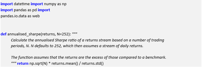
The first task is to actually obtain the data and put it into a Pandas DataFrame object. In the prior chapter on securities master implementation with Python and MySQL we created a system for achieving this. Alternatively, we can make use of this simpler code to grab Google Finance data directly and put it straight into a DataFrame. At the bottom of this script I have created a function to calculate the annualised Sharpe ratio based on a time-period returns stream:

Now that we have the ability to obtain data from Google Finance and straightforwardly calculate the annualised Sharpe ratio, we can test out a buy and hold strategy for two equities. We will use Google (GOOG) from Jan 1st 2000 to Jan 1st 2013.

We can create an additional helper function that allows us to quickly see buy-and-hold Sharpe across multiple equities for the same (hardcoded) period:

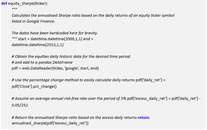
For Google, the Sharpe ratio for buying and holding is 0.703:

Now we can try the same calculation for a market-neutral strategy. The goal of this strategy is to fully isolate a particular equity’s performance from the market in general. The simplest way to achieve this is to go short an equal amount (in dollars) of an Exchange Traded Fund (ETF) that is designed to track such a market. The most obvious choice for the US large-cap equities market is the S&P500 index, which is tracked by the SPDR ETF, with the ticker of SPY.

To calculate the annualised Sharpe ratio of such a strategy we will obtain the historical prices for SPY and calculate the percentage returns in a similar manner to the previous stocks, with the exception that we will not use the risk-free benchmark. We will calculate the net daily returns which requires subtracting the difference between the long and the short returns and then dividing by 2, as we now have twice as much trading capital. Here is the Python/pandas code to carry this out:

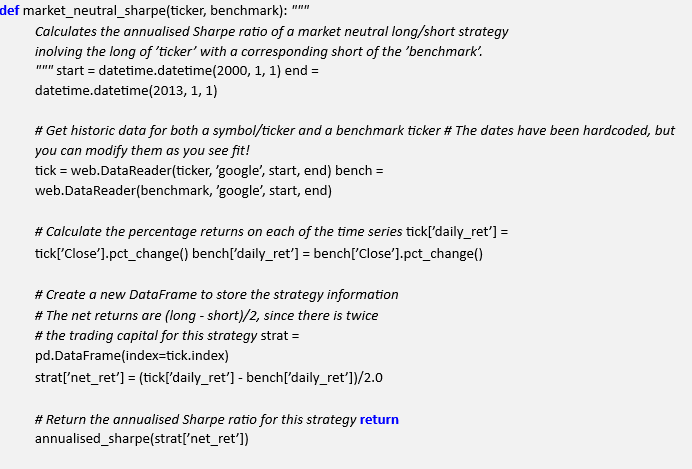
For Google, the Sharpe ratio for the long/short market-neutral strategy is 0.832:

We will now briefly consider other risk/reward ratios.

Sortino Ratio

The Sortino ratio is motivated by the fact that the Sharpe ratio captures both upward and downward volatility in its denominator. However, investors (and hedge fund managers) are generally not too bothered when we have significant upward volatility! What is actually of interest from a risk management perspective is downward volatility and periods of drawdown.

Thus the Sortino ratio is defined as the mean excess return divided by the mean downside deviation:

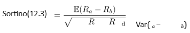
The Sortino is sometimes quoted in an institutional setting, but is certainly not as prevalent as the Sharpe ratio.

CALMAR Ratio

One could also argue that investors/traders are concerned solely with the maximum extent of the drawdown, rather than the average drawdown. This motivates the CALMAR (CALifornia Managed Accounts Reports) ratio, also known as the Drawdown ratio, which provides a ratio of mean excess return to the maximum drawdown:

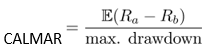
Once again, the CALMAR is not as widely used as the Sharpe ratio.

2.3]Drawdown Analysis:

In my opinion the concept of drawdown is the most important aspect of performance measurement for an algorithmic trading system. Simply put, if your account equity is wiped out then none of the other performance metrics matter! Drawdown analysis concerns the measurement of drops in account equity from previous high water marks. A high water mark is defined as the last account equity peak reached on the equity curve.

In an institutional setting the concept of drawdown is especially important as most hedge funds are remunerated only when the account equity is continually creating new high water marks. That is, a fund manager is not paid a performance fee while the fund remains “under water”, i.e. the account equity is in a period of drawdown.

Most investors would be concerned at a drawdown of 10% in a fund, and would likely redeem their investment once a drawdown exceeds 30%. In a retail setting the situation is very different. Individuals are likely to be able to suffer deeper drawdowns in the hope of gaining higher returns.

Maximum Drawdown and Duration

The two key drawdown metrics are the maximum drawdown and the drawdown duration. The first describes the largest percentage drop from a previous peak to the current or previous trough in account equity. It is often quoted in an institutional setting when trying to market a fund. Retail traders should also pay significant attention to this figure. The second describes the actual duration of the drawdown. This figure is usually quoted in days, but higher frequency strategies might use a more granular time period.

In backtests these measures provide some idea of how a strategy might perform in the future. The overall account equity curve might look quite appealing after a calculated backtest. However, an upward equity curve can easily mask how difficult previous periods of drawdown might actually have been to experience.

When a strategy begins dropping below 10% of account equity, or even below 20%, it requires significant willpower to continue with the strategy, despite the fact that the strategy may have historically, at least in the backtests, been through similar periods. This is a consistent issue with algorithmic trading and systematic trading in general. It naturally motivates the need to set prior drawdown boundaries and specific rules, such as an account-wide “stop loss” that will be carried out in the event of a drawdown breaching these levels.

Drawdown Curve

While it is important to be aware of the maximum drawdown and drawdown duration, it is significantly more instructive to see a time series plot of the strategy drawdown over the trading duration.

Fig 2.3 quite clearly shows that this particular strategy suffered from a relatively sustained period of drawdown beginning in Q3 of 2010 and finishing in Q2 of 2011, reaching a maximum drawdown of 14.8%. While the strategy itself continued to be significantly profitable over the long term, this particular period would have been very difficult to endure. In addition, this is the maximum historical drawdown that has occured to date. The strategy may be subject to an even greater drawdown in the future. Thus it is necessary to consider drawdown curves, as with other historical looking performance measures, in the context with which they have been generated, namely via historical, and not future, data.

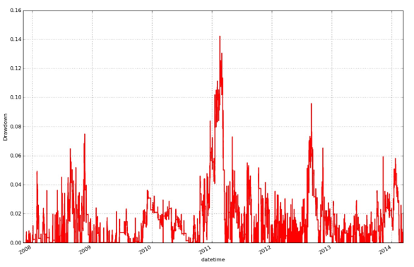
Figure 2: Typical intraday strategy drawdown curve

In the following chapter we will consider the concept of quantitative risk management and describe techniques that can help us to minimise drawdowns and maximise returns, all the while keeping to a reasonable degree of risk.