Algorithmic Trading Strategy
1.) ALGORITHMS AND ALGORITHMIC TRADING STRATEGIES
An algorithm is any well-defined computational procedure that takes values as an input and produces values as output (Cormen et al). In short, an algorithm is a set of instructions written by someone for accomplishing a given task (Johnson). Cormen et al. compares algorithms with computer hardware in a way that they believe algorithms are technologies. The authors continue stating that total system performance depends on choosing efficient algorithms as much as on choosing fast hardware. Algorithms are at the core of most technologies used in contemporary computers and quantitative trading is no different.
Algorithmic trading strategies are any form of trading in financial instruments using algorithms to automate all or some part of the trade cycle (Treleaven et al). Although automatization of trading takes place with limited or no human intervention (European Central Bank), the development of trading algorithms usually involves learning, dynamics, planning, reasoning, and decision (Treleaven et al). Furthermore, Narang , in his Strategy “Inside The black box, the simple truth about quantitative trading, ”… defines algorithmic trading strategies as a product of systematic implementation of trading strategies created by rigorous research.
The financial markets, in general, are pacified that the implementation of automated trading systems brings benefits and advantages compared with manual trading. The European Central Bank, in an article released in early 2019, acknowledged that algorithmic trading facilitates the trading process by reducing labor and other related costs. Thus, that the automatization of trading permits large volumes of data to be analyzed in very short time frames (European Central Bank).
Narang agrees and goes even further in his analysis. The author believes that with the use of a computerized, systematic implementation, traders eliminate “…decisions driven by emotion, indiscipline, passion, greed, and fear from the investment process.” Moreover, he enhances three reasons why the practice of developing algorithmic trading strategies should be highly considered for traders to be adopted; that is the benefit of deep thought, the measurement and mismeasurement of risk, and the disciplined implementation.
The benefit of deep thought
Although computers are powerful tools, they can achieve nothing without absolute precise instruction. Because of that, traders are forced to think deeply about many aspects of their strategy. In this order, an enormous amount of effort on the part of the developer is required to make a computer implement a “black-box trading strategy”.
The measurement and Mismeasurement of Risk
Rather than accepting accidental risks, the disciplined trader attempts to isolate exactly what his edge is and focus his risk taking on those areas that isolate this edge. To isolate these risks, the trader must first get an idea of what these risks are and how to measure them.
Disciplined Implementation
Perhaps the clearest characteristic one can learn from algorithmic trading strategies users comes from the discipline inherent to their approach. This is important because one of the biggest reasons that drives traders to failure is the lack of discipline. Narang argues that discretionary investors often find it exceedingly difficult to realize losses, whereas they are quick to realize gains. This is a well-documented behavioral bias known as the disposition effect. Computers, on the other hand, are not subject to this bias.
2.) ALGORITHMS AND THE FINANCIAL MARKETS
Although the financial world assents about the benefits and advantages of algorithmic trading, they seem to have different opinions on the size of trading operations executed by algorithms in the financial markets. The European Central Bank, (2019) believes that algorithmic trading has been growing continually since the early 2000s and estimates that algorithmic trading in some markets is responsible for around 70% of total orders of U.S. equity volumes. Treleaven et al. (2013) agree when they state that algorithms account for 73% of the trading volumes.
These numbers, however, diverge from other authors. For instance, Mukerji et al (2019) believe that algorithmic trading in U.S. stock market is responsible for no less than 85% of dollar trading volume – starting from the mid-1990s when algorithmic trading represented no more than 3 % of the volume traded volumes (Mukerji et al., 2019). Some estimates that automated trading accounts for over onethird of the trading volume in the United States alone (Chan, 2009b). This divergence is understandable because usually financial institutions and private traders do not disclose their information about their trading systems. However, they all agree that the use of automated systems to execute trades is growing at an astounding pace. The evolution of algorithms indicates that it is paramount that traders, investment banks, or other financial enterprises that do not yet use algorithms should upgrade their trading operations to survive in the future.
3.) UNDERSTANDING A BASIC STRUCTURE OF AN ALGORITHMIC TRADING SYSTEM
Rishi K. Narang’s Strategy, “Inside the Black Box: the simple truth about quantitative trading,” published in 2010, provides the very foundation of the structure of the algorithmic trading strategy system that is going to be used in this work. An alpha model, a risk model, and a transaction cost model are the three main modules that compound the basic structure of an algorithm trading system. These modules produce information that feeds a portfolio construction model, which in turn interacts with the execution model.
While alpha models are the part of the algorithm designed to forecast the price of the asset the trader wants to consider trading for the goal of generating returns, Risk models are developed to limit exposures that could lead traders to losses. Transaction cost models are used to identify the cost of opening or closing new trading positions.
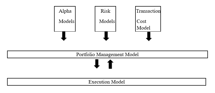
Figure 3.1– Basic Structure of an Algorithmic Trading System
Portfolio construction modules ponder the outputs from the alpha, risk, and transaction costs modules, determining the best portfolio to hold. Finally, the execution model initiates the process to execute the order to buy or sell the asset analyzed by the system.
3.1] Alpha Models:
Alpha models may be the main model of a trading strategy algorithm and where the research process is focused. Because they hold as core premise that no instrument is inherently good or bad they have projected to time the selection and/or sizing of portfolio holdings.
A few synonyms for an alpha model are forecasts, factors, alphas, models, strategies, estimators, or predictors. All successful alpha models are developed in a way that allows them to predict the future well enough that, after allowing for them to lose money in a few trades, they can still be profitable in the long run. Narang continuously stated that “…of the various parts of a quants strategy, the alpha model is the optimist, focused on making money by predicting the future.”.
3.1.1) Types of Alpha Models: Theory Driven and Data Driven:
For a trader seeking alpha, there are a small number of basic trading strategies available that can be implemented in several ways. Understanding the perspectives quantitative traders take on science is an important element in understanding quantitative trading strategies.
Theoretical and empirical are the two major branches of science. The theoretical branch tries to make sense of the world around them by hypothesizing why it is the way it is. The empirical branch believes that enough data from the environment is enough to predict future patterns of behavior, even if there is no hypothesis to rationalize the behavior in an intuitive way.
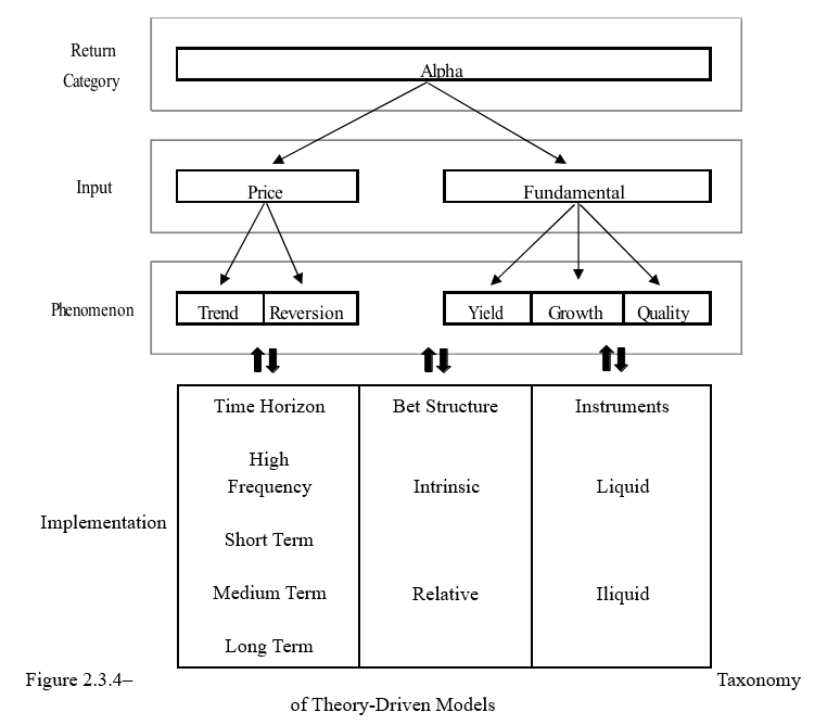
Narang points that most of the quantitative traders are theory-driven and most of what they do can be fit into one of five categories of phenomena: trend, reversion, value/yield, growth, and quality, which can be understood by examining price-related data or fundamental data. Perceiving the inputs to a strategy is paramount to understanding the strategy itself. Trend and mean reversion trading strategies rely on price-related data while value/yield, growth, and quality trading strategies are based on fundamental data.
Traders who seek to predict prices and to profit from such predictions are likely to be using one of two kinds of phenomena. The first idea, trend following or momentum, is that, once started, an trend will continue, and the second idea, which we call counter-trend or mean reversion, is that the trend will, anywhere in the future, reverse.
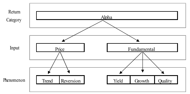
Figure 3.2– A Taxonomy of Theory-Driven Alpha Models
Trend Following
Trend following happens to be the oldest of all quantitative trading strategies. Ed Seykota built the first computerized version of the mechanical trend-following strategy that Richard Donchian created some years earlier, utilizing punch cards on an IBM mainframe in 1970.
Trend following strategies are based on the theory that asset prices from time to time move in the same direction for a period sufficiently long that a trader can identify this trend and ride it. The economic theory that supports the existence of trends is based on the understanding of consensusbuilding among market participants.
An alternative explanation of the motive trends that happen is known as the greater fools’ theory. The idea is that, by the simple fact that traders believe in trend, they tend to start buying any asset whose price is going up and selling any asset whose price is going down, which itself perpetuates the trend.
As trend followers tend to search for a meaningful move in a given direction in an instrument, one way to identify a trend for trading purposes, for instance, is to use a moving average crossover indicator. This tool compares the average price of the index over a shorter period (i.e., 50 days – the red line showed in figure 3) to that of a longer period (i.e., 200 days – the blue line shown in Figure 2.3.3). When the shorter-term average price crosses downward the longer-term average price, the index is said to be in a negative trend. On the opposite way, when the shorter- term average price crosses upward the longer-term average, the index is in a positive trend. Figure 3.3 gives us examples of a few entries a trader could have used the average crossover strategy.
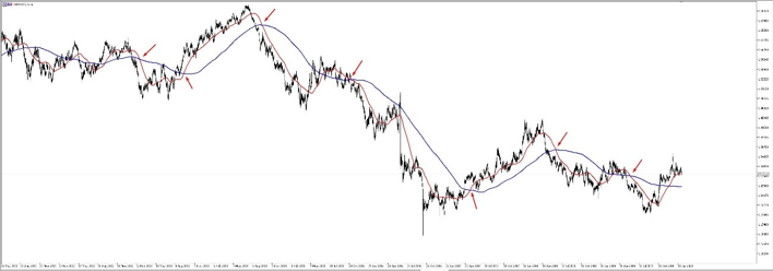
Figure 3.3– GBPUSD Daily Chart with Moving Averages (MA 50 & MA 200) Indicator
Mean Reversion
Traders practicing mean reversion strategies, also known as contrarians, believe that exists a center of gravity around which prices fluctuate. With this theory, a trader could identify both this center of gravity and the range around this center to warrant making a trade. One of the rationales behind this theory is that exists short-term imbalances among buyers and sellers due to liquidity.
Because short-term oscillations occur around longer-term trend, trend and mean reversion strategies are not always at odds with other. Mean reversion traders, after identifying the current equilibrium point of the oscillation, must determine the amount of divergence from that equilibrium is enough to make a trade feasible. Statistical arbitrage, which bets on the convergence of the prices of similar assets whose prices have diverged, is probably the best example of a mean reversion strategy.
Trend and mean reversion strategies, although they are theoretically opposite ideas, represent a large portion of all quantitative trading because they seem to work well in different timeframes. While trends occur in higher horizons, reversions tend to happen over short-term horizons.
3.1.2) Strategies Utilizing Fundamental Data:
Value/Yield
Although this idea is used in other markets, value strategies, also known as earning yield, are usually associated with equity trading. The main idea of values strategies is that the higher the yield, the cheaper the instrument. Of the many metrics used to define value, price-to-earning (P/E) is one of the most common of them. To avoid division by zero, which could cause a dramatic error in the algorithm, quantitative traders, however, tend to invert the ratio, keeping prices in the denominator.
One of the most popular value strategies among currencies quantitative traders is the carry trade strategy. The logic of this strategy is to purchase the currency of one country with higher short-term yields against a short position in the currency of a country with relatively low short-term yields.
Growth
The goal of growth strategies is to search predictions based on an asset’s expected or historically observed level of economic growth. The gross domestic product (GDP) of a country or the earning growth of a company are good examples of that. The theory behind this idea is that, ceteris paribus, it is better to sell assets that are experiencing slow or negative growth or sell assets that are experiencing slow or negative growth.
Quality
Investors that pursue this quality strategy believe that, ceteris paribus, it is preferable to go long on assets that are of high quality to their portfolios and/or to go short on poor quality assets. The idea of this strategy is that, on one side, capital safety is important, and, on the other side, neither growth nor value strategies can identify this concept.
3.1.3) Data-Driven Alpha Models:
The premise of Data mining is that data will most predict price movement based on some patterns recognizable through analytical techniques. One advantage of this technique is when compared with theory-driven strategies, data mining is technically more challenging and far less widely practiced. Another advantage is that data-driven strategies can identify behaviors whether they have been identified before by some theory or not. This means that these models can see events without having to understand why they happen.
Data-driven alpha models work better in short-term time horizons (i.e., minutes or less). This happens because, at this timescale, the quantity of data available can be so vast that the researcher has a better chance of finding statistically significant results in his testing.
The quantitative trader willing to practice this strategy, however, should be aware of two shortcomings. The first one is that the researcher must carefully decide what data to feed the model. The amount of data searching the algorithms, if not chosen well, could be so enormous that a huge and expensive hardware structure would be necessary to predict anything in time to make the trade. The second problem is that the generation of alphas with the use of data-mining alone could lead to false signals that act like “traps for data miners”.
3.2] Risk Models
An attentive trader should not worry only about the avoidance of risk or reduction of loss. In addition to these goals, the intentional selection and sizing of exposures to improve the quality and consistency of returns are most essential for its survival in the financial markets. Risk exposures will most likely not produce profits over the long run; however, they can seriously undermine the returns of a strategy over time. Furthermore, any attempt to forecast these risk exposures should be avoided simply because they cannot be predicted successfully. What matters is the ability to understand and measure several exposures and to be intentional about the selection of such exposures.
The idea is that alpha models and risk models should present opposite perspectives. For example, if alpha models present a high probability forecast, risk models would largely control the size of desirable exposures or deal with undesirable types of exposures.
Risk management involves some knowledge on the monetary amount the trader is willing to risk in addition to the amount it is aiming to profit. Without the sense of it, traders hold on losing positions longer than they should of close profitable positions too soon (Lien). The result, continues Lien, is that the trader ends up with a negative profit/loss relation (P/L), although he may have had more winning positions than losing positions.
From the many types of risk models available, there are three main ways that a trader can have their approach in risk management. Authors, such as Basso, Lien, and Narang, defend that position size limiting, risk-reward ratio, and stop-loss order represents a high degree of importance for risk management.
Limiting the size or eliminating it can work as an alternative to just accepting a given type of exposure. The trader, now in the role of a risk manager, should determine which of these courses of action is appropriate for each kind of exposure and feed the risk model to assess if the trade is worth taking or not.
How size is limited can be mainly approached by constraint or penalty forms. Hard constraints, as the name suggests, are set to establish a fixed position in terms of risk (Basso). For example, no position should be larger than 3% of the account balance, however, because the distance from the entry price to the stop-loss order price vary from trade to trade, the contract size of the position is adjusted so the risk does not increase. The penalty function work in a way that will allow a position to be greater than 3% but will impose heavier penalties to allow that. These penalties through research can be determined either from the data or from theory.
Setting a risk-reward ratio to trading strategies is a powerful tool to keep a positive profit and loss ratio and to prevent traders from opening positions that ultimately are not worth the risk. It allows the strategy to have an exact amount of how much profit the trade should achieve against the amount risked opening the position (Lien). Thus, the risk-reward ratio varies from strategy to strategy, but as a ‘rule of thumb’, according to Lien, it should be no less than 1:2.
Finally, Stop-loss orders, alongside with risk size limiting and risk-reward ratio, are essencial to control your losses, in line with position risk size. Setting the limit to your losses avoids the common predicament of being in a scenario where strategies have a high probability of profitable trades but a loss large enough to give all the profit back to the market (Basso). Thus, the author suggests that it is a good habit to move the stop-loss order to the break-even level as soon as the position has profited by the same amount initially risked for the trade. She also points that some strategies choose to close a portion of the position once profit equals the amount risked.
Managing risk daily basis not only can reduce the volatility of the return of a strategy, but also, and far more important, can reduce the likelihood of large losses. In many cases, the failures of some quantitative traders are directed associated with failures to manage risk.
3.3] Transaction Cost Models:
Narang describes a transaction cost model as “a way of quantifying the cost of making a trade of a given size so that this information can be used in conjunction with the alpha and risk models to determine the best portfolio to hold.” The model will decide if the cost of opening a position is worth it or not. Furthermore, on one hand, if the cost of transacting is underestimated, the algorithm could be led to make too many trades that would have insufficient benefit. On the other hand, overestimating the cost of transacting could lead the algorithm to miss trading opportunities or to hold positions too long.
Transaction cost models can be explained in two basic types: flat, linear, piecewise-linear, and quadratic. A flat transaction cost model means that the cost of trading is constant no matter the size of the order. A linear transaction cost model means that the cost grows on the same scale as that of the transaction size.
3.4) Portfolio Construction Models:
The decision to allocate assets in a portfolio is based on an equilibrium of considerations of expected return, risk, and transaction costs. Quantitative portfolio construction models are defined by a rulebased portfolio construction model, which is based on heuristics defined by the quantitative trader, and optimized portfolio construction models such as the Markowitz (1952) modern portfolio theory and the Tobin (1958) two-fund separation theorem, which utilizes step-by-step sets of rules designed to get the user from a starting point to the desired point.
4.) FOREIGN EXCHANGE MARKETS
The world’s financial markets are vast, in terms of both the size and diversity of products they incorporate. Generally speaking, the financial market can be broken down into four main categories, namely: i) capital markets; ii) foreign exchange markets; iii) money markets; and iv) derivative markets (Johnson). For the sake of simplicity, this work will focus its attention only on foreign exchange markets.
Foreign exchange markets, at their most basic level, are over-the-counter markets with no central exchange and clearing house where orders are matched. Foreign exchange dealers and markets makers around the planet are linked to each other around the clock creating one cohesive market (Lien).
As the largest and fasted markets in the world, foreign exchange markets allow traders to operate 24-hour per day, 6-days per week in a market with an average daily volume of transactions of $6,6 trillion U.S. dollars (Bank for International Settlement).
As these markets became accessible to trade by individual retail investors around twenty years ago, and because they present such attractive characteristics, foreign exchange markets exploded in popularity (Lien).
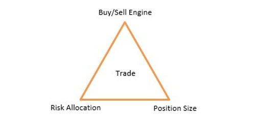
5.) POSITION SIZING AND RISK ALLOCATION
The establishment of the volume of trade, along with the Buy/Sell Engine, which is the entry-level and the stop-loss size, and the maximum risk allocation for a trade, makes up the structural tripod for risk management in trading operations (Basso).
Among different forms available of calculating it, Basso provides two popular techniques to calculate the volume for a single trade. The first one uses the monetary value of the risk of the trade has a divisor, which is the difference between the current bid/ask price and the stop-loss limit price stablished for that single trade – see formula (1). The second technique utilizes the Average True Range (ATR) indicator, which measures the volatility of a specific asset in a given period – see formula (2).
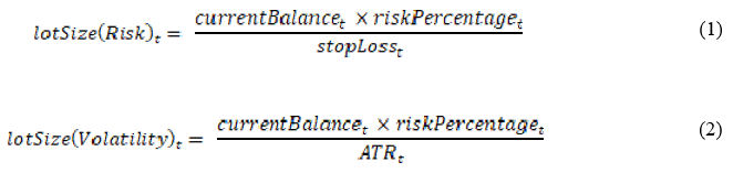
Where, currentBalance is the monetary value of the equity in the account at the moment of the trade, riskPercentage is the current portfolio risk in percentage allocated to a single position, stopLoss is the monetary risk on the upcoming trade, and ATR is the average True Range indicator value.
Concerning risk allocation, there is no consensus in the literature for the definition of a fixed value corresponding to a maximum risk, in percentages, to allocate in a single trade. (Narang), suggests the amount of 3% of the current portfolio equity, allowing the automated system to raise the risk allocation to 5% if the alpha model emits a strong signal. Basso, on the other hand, proposes that maximum risks could vary from 0.5% to 2% of the account balance, depending on the trader’s appetite for risk.
6.) TECHNICAL INDICATORS
Over time, although traders have been developing and using technical indicators to aid them in the prediction of price movements in the various markets, the topic has received significantly less attention in the literature (Neely et al). Technical indicators are heuristic or pattern-based signals that rely on past price, volume patterns, or/and open interest of an asset to identify price trends believed to persist into the future; see James and Neely et al. for recent surveys.
6.1] Moving Average Indicator:
As one of the first trading tools ever invented (Narang), and because of its simplicity and intuitive appeal (Guo et al.), the moving average (MA) is one of the most popular technical indicators (Zhu & Zhou). The MA is a technical analysis tool that smooths out price data over a specific period by creating a constantly updated average price (Cory). The common moving average formula is given by;
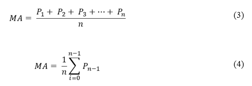
Where MA is the moving average value, Pn is the price of an asset at period n-1, and n is the number of total periods.
6.2] Average Directional Index Indicator:
Created by (Wilder Jr.), the Average Directional Index (ADX) is a trend-following technical analysis indicator that some traders use to determine the strength, or the magnitude, of a trend (Mitchell), but not the actual direction of the later. It is used together with an positive directional indicator (DI+) and a negative directional indicator (DI-), which identifies if there is a trend (Gurrib). See formula (5). For a better understanding of the formula, see Wilder Jr. and Gurrib.
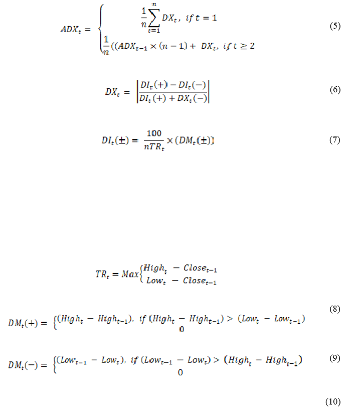
Where n is the period set to the ADX, DX is the directional index, DI(±) is the positive and negative directional indicator, DM(±) is the directional movements, and TR is the True Range indicator.
Read Also; Algo Trading Strategy Optimisation