Time Series Analysis In Algorithmic Trading

In this chapter we are going to consider statistical tests that will help us identify price series that possess trending or mean-reverting behaviour. If we can identify such series statistically then we can capitalise on this behaviour by forming momentum or mean-reverting trading strategies.

In later chapters we will use these statistical tests to help us identify candidate time series and then create algorithmic strategies around them.

1.) Testing for Mean Reversion

One of the key quantitative trading concepts is mean reversion. This process refers to a time series that displays a tendency to revert to a historical mean value. Such a time series can be exploited to generate trading strategies as we enter the market when a price series is far from the mean under the expectation that the series will return to a mean value, whereby we exit the market for a profit. Mean-reverting strategies form a large component of the statistical arbitrage quant hedge funds. In later chapters we will create both intraday and interday strategies that exploit mean-reverting behaviour.

The basic idea when trying to ascertain if a time series is mean-reverting is to use a statistical test to see if it differs from the behaviour of a random walk. A random walk is a time series where the next directional movement is completely independent of any past movements – in essence the time series has no “memory” of where it has been. A mean-reverting time series, however, is different. The change in the value of the time series in the next time period is proportional to the current value. Specifically, it is proportional to the difference between the mean historical price and the current price.

Mathematically, such a (continuous) time series is referred to as an Ornstein-Uhlenbeck process. If we can show, statistically, that a price series behaves like an Ornstein-Uhlenbeck series then we can begin the process of forming a trading strategy around it. Thus the goal of this chapter is to outline the statistical tests necessary to identify mean reversion and then use Python libraries (in particular statsmodels) in order to implement these tests. In particular, we will study the concept of stationarity and how to test for it.

As stated above, a continuous mean-reverting time series can be represented by an OrnsteinUhlenbeck stochastic differential equation:

dx_t= θ(µ − x_t)dt + σdW_t

Where θ is the rate of reversion to the mean, µ is the mean value of the process, σ is the variance of the process and W_tis a Wiener Process or Brownian Motion.

This equation essentially states that the change of the price series in the next continuous time period is proportional to the difference between the mean price and the current price, with the addition of Gaussian noise.

We can use this equation to motivate the definition of the Augmented Dickey-Fuller Test, which we will now describe.

1.1] Augmented Dickey-Fuller (ADF) Test:

The ADF test makes use of the fact that if a price series possesses mean reversion, then the next price level will be proportional to the current price level. Mathematically, the ADF is based on the idea of testing for the presence of a unit root in an autoregressive time series sample.

We can consider a model for a time series, known as a linear lag model of order p. This model says that the change in the value of the time series is proportional to a constant, the time itself and the previous p values of the time series, along with an error term:

Where α is a constant, β represents the coefficient of a temporal trend and ∆y_t= y(t) − y(t − 1). The role of the ADF hypothesis test is to ascertain, statistically, whether γ = 0, which would indicate (with α = β = 0) that the process is a random walk and thus non mean reverting.

Hence we are testing for the null hypothesis that γ = 0.

If the hypothesis that γ = 0 can be rejected then the following movement of the price series is proportional to the current price and thus it is unlikely to be a random walk. This is what we mean by a “statistical test”.

So how is the ADF test carried out?

Calculate the test statistic, DF_τ, which is used in the decision to reject the null hypothesis
Use the distribution of the test statistic (calculated by Dickey and Fuller), along with the critical values, in order to decide whether to reject the null hypothesis

Let’s begin by calculating the test statistic (DF_τ). This is given by the sample proportionality constant γˆ divided by the standard error of the sample proportionality constant:

Now that we have the test statistic, we can use the distribution of the test statistic calculated by Dickey and Fuller to determine the rejection of the null hypothesis for any chosen percentage critical value. The test statistic is a negative number and thus in order to be significant beyond the critical values, the number must be smaller (i.e. more negative) than these values.

A key practical issue for traders is that any constant long-term drift in a price is of a much smaller magnitude than any short-term fluctuations and so the drift is often assumed to be zero (β = 0) for the linear lag model described above.

Since we are considering a lag model of order p, we need to actually set p to a particular value. It is usually sufficient, for trading research, to set p = 1 to allow us to reject the null hypothesis. However, note that this technically introduces a parameter into a trading model based on the ADF.

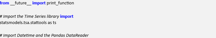
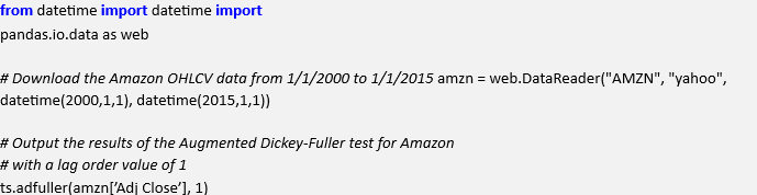
To calculate the Augmented Dickey-Fuller test we can make use of the pandas and statsmodels libraries. The former provides us with a straightforward method of obtaining Open-High-LowClose-Volume (OHLCV) data from Yahoo Finance, while the latter wraps the ADF test in a easy to call function. This prevents us from having to calculate the test statistic manually, which saves us time.

We will carry out the ADF test on a sample price series of Amazon stock, from 1st January 2000 to 1st January 2015.

Here is the Python code to carry out the test:

Here is the output of the Augmented Dickey-Fuller test for Amazon over the period. The first value is the calculated test-statistic, while the second value is the p-value. The fourth is the number of data points in the sample. The fifth value, the dictionary, contains the critical values of the test-statistic at the 1, 5 and 10 percent values respectively.

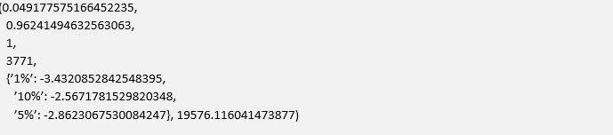
Since the calculated value of the test statistic is larger than any of the critical values at the 1, 5 or 10 percent levels, we cannot reject the null hypothesis of γ = 0 and thus we are unlikely to have found a mean reverting time series. This is in line with our tuition as most equities behave akin to Geometric Brownian Motion (GBM), i.e. a random walk.

This concludes how we utilise the ADF test. However, there are alternative methods for detecting mean-reversion, particularly via the concept of stationarity, which we will now discuss.

1.2] Testing for Stationarity:

A time series (or stochastic process) is defined to be strongly stationary if its joint probability distribution is invariant under translations in time or space. In particular, and of key importance for traders, the mean and variance of the process do not change over time or space and they each do not follow a trend.

A critical feature of stationary price series is that the prices within the series diffuse from their initial value at a rate slower than that of a GBM. By measuring the rate of this diffusive behaviour we can identify the nature of the time series and thus detect whether it is mean-reverting.

We will now outline a calculation, namely the Hurst Exponent, which helps us to characterise the stationarity of a time series.

1.2.1) Hurst Exponent:

The goal of the Hurst Exponent is to provide us with a scalar value that will help us to identify (within the limits of statistical estimation) whether a series is mean reverting, random walking or trending.

The idea behind the Hurst Exponent calculation is that we can use the variance of a log price series to assess the rate of diffusive behaviour. For an arbitrary time lag τ, the variance of τ is given by:

Var(τ) = h|log(t + τ) − log(t)|²i

Where the brackets h and i refer to the average over all values of t.

The idea is to compare the rate of diffusion to that of a GBM. In the case of a GBM, at large times (i.e. when τ is large) the variance of τ is proportional to τ:

h|log(t + τ) − log(t)|²i ∼ τ

If we find behaviour that differs from this relation, then we have identified either a trending or a mean-reverting series. The key insight is that if any sequential price movements possess non-zero correlation (known as autocorrelation) then the above relationship is not valid. Instead it can be modified to include an exponent value “2H“, which gives us the Hurst Exponent value H:

h|log(t + τ) − log(t)|²i ∼ τ^2H

Thus it can be seen that if H = 0.5 we have a GBM, since it simply becomes the previous relation. However if H 6= 0.5 then we have trending or mean-reverting behaviour. In particular:

H < 0.5 – The time series is mean reverting
H = 0.5 – The time series is a Geometric Brownian Motion
H > 0.5 – The time series is trending

In addition to characterisation of the time series the Hurst Exponent also describes the extent to which a series behaves in the manner categorised. For instance, a value of H near 0 is a highly mean reverting series, while for H near 1 the series is strongly trending.

To calculate the Hurst Exponent for the Amazon price series, as utilised above in the explanation of the ADF, we can use the following Python code:

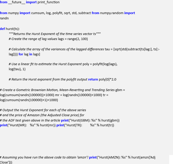
The output from the Hurst Exponent Python code is given below:

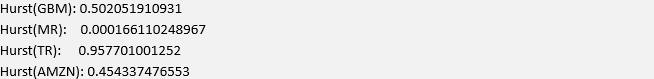
From this output we can see that the GBM possesses a Hurst Exponent, H, that is almost exactly 0.5. The mean reverting series has H almost equal to zero, while the trending series has

H close to 1.

Interestingly, Amazon has H also close to 0.5 indicating that it is similar to a GBM, at least for the sample period we’re making use of!

3.) Cointegration

It is actually very difficult to find a tradable asset that possesses mean-reverting behaviour. Equities broadly behave like GBMs and hence render the mean-reverting trade strategies relatively useless. However, there is nothing stopping us from creating a portfolio of price series that is stationary. Hence we can apply mean-reverting trading strategies to the portfolio.

The simplest form of mean-reverting trade strategies is the classic “pairs trade”, which usually involves a dollar-neutral long-short pair of equities. The theory goes that two companies in the same sector are likely to be exposed to similar market factors, which affect their businesses. Occasionally their relative stock prices will diverge due to certain events, but will revert to the long-running mean.

Let’s consider two energy sector equities Approach Resources Inc given by the ticker AREX and Whiting Petroleum Corp given by the ticker WLL. Both are exposed to similar market conditions and thus will likely have a stationary pairs relationship. We are now going to create some plots, using pandas and the Matplotlib libraries to demonstrate the cointegrating nature of AREX and WLL. The first plot (Figure 10.1) displays their respective price histories for the period Jan 1st 2012 to Jan 1st 2013.

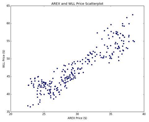
If we create a scatter plot of their prices, we see that the relationship is broadly linear (see Figure 10.2) for this period.

The pairs trade essentially works by using a linear model for a relationship between the two stock prices:

Where y(t) is the price of AREX stock and x(t) is the price of WLL stock, both on day t.

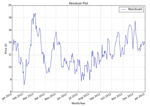
If we plot the residuals (for a particular value of β that we will determine below) we create a new time series that, at first glance, looks relatively stationary. This is given in Figure 10.3.

We will describe the code for each of these plots below.

3.1] Cointegrated Augmented Dickey-Fuller Test:

In order to statistically confirm whether this series is mean-reverting we could use one of the tests we described above, namely the Augmented Dickey-Fuller Test or the Hurst Exponent. However, neither of these tests will actually help us determine β, the hedging ratio needed to form the linear combination, they will only tell us whether, for a particular β, the linear combination is stationary.

This is where the Cointegrated Augmented Dickey-Fuller (CADF) test comes in. It determines the optimal hedge ratio by performing a linear regression against the two time series and then tests for stationarity under the linear combination.

Figure 1: Time series plots of AREX and WLL

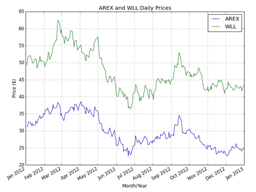
Figure 2: Scatter plot of AREX and WLL prices

Python Implementation

We will now use Python libraries to test for a cointegrating relationship between AREX and WLL for the period of Jan 1st 2012 to Jan 1st 2013. We will use Yahoo Finance for the data source and Statsmodels to carry out the ADF test, as above.

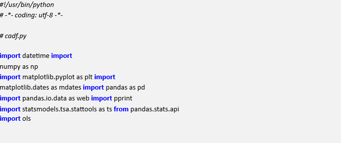
The first task is to create a new file, cadf.py, and import the necessary libraries. The code makes use of NumPy, Matplotlib, Pandas and Statsmodels. In order to correctly label the axes Figure 10.3: Residual plot of AREX and WLL linear combination.

and download data from Yahoo Finance via pandas, we import the matplotlib.dates module and the pandas.io.data module. We also make use of the Ordinary Least Squares (OLS) function from pandas:

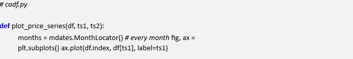
The first function, plot_price_series, takes a pandas DataFrame as input, with to columns given by the placeholder strings “ts1” and “ts2”. These will be our pairs equities. The function simply plots the two price series on the same chart. This allows us to visually inspect whether any cointegration may be likely.

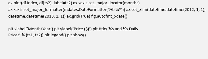
We use the Matplotlib dates module to obtain the months from the datetime objects. Then we create a figure and a set of axes on which to apply the labelling/plotting. Finally, we plot the figure:

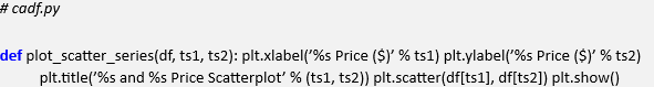
The second function, plot_scatter_series, plots a scatter plot of the two prices. This allows us to visually inspect whether a linear relationship exists between the two series and thus whether it is a good candidate for the OLS procedure and subsequent ADF test:

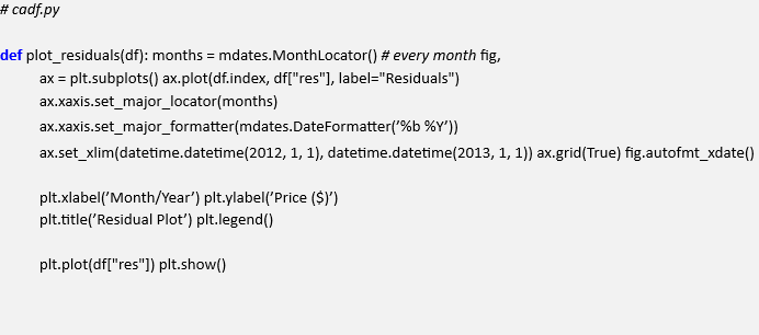
The third function, plot_residuals, is designed to plot the residual values from the fitted linear model of the two price series. This function requires that the pandas DataFrame has a “res” column, representing the residual prices:

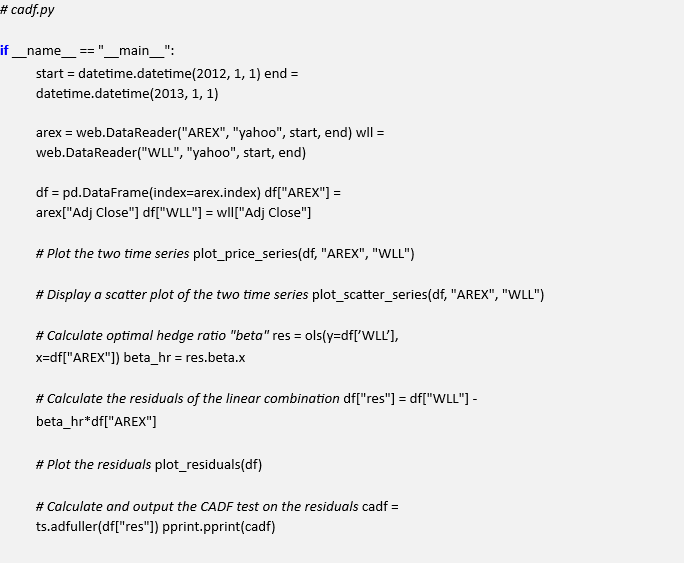
Finally, the procedure is wrapped up in a __main__ function. The first task is to download the OHLCV data for both AREX and WLL from Yahoo Finance. Then we create a separate DataFrame, df, using the same index as the AREX frame to store both of the adjusted closing price values. We then plot the price series and the scatter plot.

After the plots are complete the residuals are calculated by calling the pandas ols function on the WLL and AREX series. This allows us to calculate the β hedge ratio. The hedge ratio is then used to create a “res” column via the formation of the linear combination of both WLL and AREX.

Finally the residuals are plotted and the ADF test is carried out on the calculated residuals. We then print the results of the ADF test:

The output of the code (along with the Matplotlib plots) is as follows:

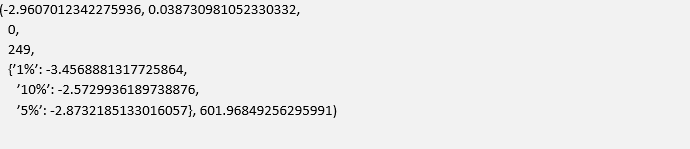
It can be seen that the calculated test statistic of -2.96 is smaller than the 5% critical value of -2.87, which means that we can reject the null hypothesis that there isn’t a cointegrating relationship at the 5% level. Hence we can conclude, with a reasonable degree of certainty, that AREX and WLL possess a cointegrating relationship, at least for the time period sample considered.

We will use this pair in subsequent chapters to create an actual trading strategy using an implemented event-driven backtesting system.

4.) Why Statistical Testing?

Fundamentally, as far as algorithmic trading is concerned, the statistical tests outlined above are only as useful as the profits they generate when applied to trading strategies. Thus, surely it makes sense to simply evaluate performance at the strategy level, as opposed to the price/time series level? Why go to the trouble of calculating all of the above metrics when we can simply use trade level analysis, risk/reward measures and drawdown evaluations?

Firstly, any implemented trading strategy based on a time series statistical measure will have a far larger sample to work with. This is simply because when calculating these statistical tests, we are making use of each bar of information, rather than each trade. There will be far less round-trip trades than bars and hence the statistical significance of any trade-level metrics will be far smaller.

Secondly, any strategy we implement will depend upon certain parameters, such as lookback periods for rolling measures or z-score measures for entering/exiting a trade in a meanreversion setting. Hence strategy level metrics are only appropriate for these parameters, while the statistical tests are valid for the underlying time series sample.

In practice we want to calculate both sets of statistics. Python, via the statsmodels and pandas libraries, make this extremely straightforward. The additional effort is actually rather minimal!