Quantitative Trading: Exploring Promising Strategies and Their Hidden Risks

Exploring Promising Strategies and Their Hidden Risks

Now, let’s suppose that you have read about several potential strategies that fit your personal requirements. Presumably, someone else has done backtests on these strategies and reported that they have great historical returns. Before proceeding to devote your time to performing a comprehensive backtest on this strategy (not to mention devoting your capital to actually trading this strategy), there are a number of quick checks you can do to make sure you won’t be wasting your time or money.

How Does It Compare with a Benchmark and How Consistent Are Its Returns?

This point seems obvious when the strategy in question is a stock trading strategy that buys (but not shorts) stocks. Everybody seems to know that if a long-only strategy returns 10 percent a year, it is not too fantastic because investing in an index fund will generate as much, if not better, return on average. However, if the strategy is a long-short dollar-neutral strategy (i.e., the portfolio holds long and short positions with equal capital), then 10 percent is quite a good return, because then the benchmark of comparison is not the market index, but a riskless asset such as the yield of the three-month U.S. Treasury bill (which at the time of this writing is about 4 percent).

Another issue to consider is the consistency of the returns generated by a strategy. Though a strategy may have the same average return as the benchmark, perhaps it delivered positive returns every month while the benchmark occasionally suffered some very bad months. In this case, we would still deem the strategy superior. This leads us to consider the information ratio or Sharpe ratio (Sharpe, 1994), rather than returns, as the proper performance measurement of a quantitative trading strategy.

Information ratio is the measure to use when you want to assess a long-only strategy. It is defined as;

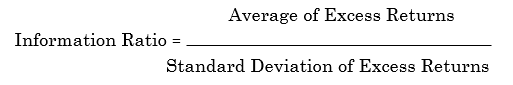
where;

Now the benchmark is usually the market index to which the securities you are trading belong. For example, if you trade only small-cap stocks, the market index should be the Standard & Poor’s small-cap index or the Russell 2000 index, rather than the S&P 500. If you are trading just gold futures, then the market index should be gold spot price, rather than a stock index.

The Sharpe ratio is actually a special case of the information ratio, suitable when we have a dollar-neutral strategy, so that the benchmark to use is always the risk-free rate. In practice, most traders use the Sharpe ratio even when they are trading a directional (long or short only) strategy, simply because it facilitates comparison across different strategies. Everyone agrees on what the risk free rate is, but each trader can use a different market index to come up with their own favorite information ratio, rendering comparison difficult.

(Actually, there are some subtleties in calculating the Sharpe ratio related to whether and how to subtract the risk-free rate, how to annualize your Sharpe ratio for ease of comparison, and so on. I will cover these subtleties in the next chapter, which will also contain an example on how to compute the Sharpe ratio for a dollar-neutral and a long-only strategy.)

If the Sharpe ratio is such a nice performance measure across different strategies, you may wonder why it is not quoted more often instead of returns. In fact, when a colleague and I went to SAC Capital Advisors (assets under management: $14 billion) to pitch a strategy, their then head of risk management said to us: “Well, a high Sharpe ratio is certainly nice, but if you can get a higher return instead, we can all go buy bigger houses with our bonuses!” This reasoning is quite wrong: A higher Sharpe ratio will actually allow you to make more profits in the end, since it allows you to trade at a higher leverage. It is the leveraged return that matters in the end, not the nominal return of a trading strategy. For more on this, see Blog on money and risk management.

(And no, our pitching to SAC was not successful, but for reasons quite unrelated to the returns of the strategy. In any case, at that time neither my colleague nor I were familiar enough with the mathematical connection between the Sharpe ratio and leveraged returns to make a proper counterargument to that head of risk management.)

Now that you know what a Sharpe ratio is, you may want to find out what kind of Sharpe ratio your candidate strategies have. Often, they are not reported by the authors of that strategy, and you will have to e-mail them in private for this detail. And often, they will oblige, especially if the authors are finance professors; but if they refuse, you have no choice but to perform the backtest yourself. Sometimes, however, you can still make an educated guess based on the flimsiest of information:

If a strategy trades only a few times a year, chances are its Sharpe ratio won’t be high. This does not prevent it from being part of your multi-strategy trading business, but it does disqualify the strategy from being your main profit center.

If a strategy has deep (e.g., more than 10 percent) or lengthy (e.g., four or more months) drawdowns, it is unlikely that it will have a high Sharpe ratio. I will explain the concept of drawdown in the next section, but you can just visually inspect the equity curve (which is also the cumulative profit-and-loss curve, assuming no redemption or cash infusion) to see if it is very bumpy or not. Any peak-to-trough of that curve is a drawdown. (See Figure.1 for an example.)

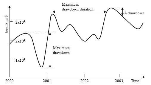
FIGURE.1 Drawdown, Maximum Drawdown, and Maximum Drawdown Duration

As a rule of thumb, any strategy that has a Sharpe ratio of less than 1 is not suitable as a stand-alone strategy. For a strategy that achieves profitability almost every month, its (annualized) Sharpe ratio is typically greater than 2. For a strategy that is profitable almost every day, its Sharpe ratio is usually greater than 3. I will show you how to calculate Sharpe ratios for various strategies.

How Deep and Long Is the Drawdown?

A strategy suffers a drawdown whenever it has lost money recently. A drawdown at a given time t is defined as the difference between the current equity value (assuming no redemption or cash infusion) of the portfolio and the global maximum of the equity curve occurring on or before time t. The maximum drawdown is the difference between the global maximum of the equity curve with the global minimum of the curve after the occurrence of the global maximum (time order matters here: The global minimum must occur later than the global maximum). The global maximum is called the “high watermark.” The maximum drawdown duration is the longest it has taken for the equity curve to recover losses.

More often, drawdowns are measured in percentage terms, with the denominator being the equity at the high watermark, and the numerator being the loss of equity since reaching the high watermark.

Figure.1 illustrates a typical drawdown, the maximum drawdown, and the maximum drawdown duration of an equity curve. I will include a tutorial on how to compute these quantities from a table of daily profits and losses using either Excel or MATLAB. One thing to keep in mind: The maximum drawdown and the maximum drawdown duration do not typically overlap over the same period.

Defined mathematically, drawdown seems abstract and remote. However, in real life there is nothing more gut-wrenching and emotionally disturbing to suffer than a drawdown if you’re a trader. (This is as true for independent traders as for institutional ones. When an institutional trading group is suffering a drawdown, everybody seems to feel that life has lost meaning and spend their days dreading the eventual shutdown of the strategy or maybe even the group as a whole.) It is therefore something we would want to minimize. You have to ask yourself, realistically, how deep and how long a drawdown will you be able to tolerate and not liquidate your portfolio and shut down your strategy? Would it be 20 percent and three months, or 10 percent and one month? Comparing your tolerance with the numbers obtained from the backtest of a candidate strategy determines whether that strategy is for you.

Even if the author of the strategy you read about did not publish the precise numbers for drawdowns, you should still be able to make an estimate from a graph of its equity curve. For example, in Figure.1, you can see that the longest drawdown goes from around February 2001 to around October 2002. So the maximum drawdown duration is about 20 months. Also, at the beginning of the maximum drawdown, the equity was about $2.3 × 104, and at the end, about $0.5 × 104. So the maximum drawdown is about $1.8 × 104.

How Will Transaction Costs Affect the Strategy?

Every time a strategy buys and sells a security, it incurs a transaction cost. The more frequent it trades, the larger the impact of transaction costs will be on the profitability of the strategy. These transaction costs are not just due to commission fees charged by the broker. There will also be the cost of liquidity when you buy and sell securities at their market prices, you are paying the bid-ask spread. If you buy and sell securities using limit orders, however, you avoid the liquidity costs but incur opportunity costs. This is because your limit orders may not be executed, and therefore you may miss out on the potential profits of your trade. Also, when you buy or sell a large chunk of securities, you will not be able to complete the transaction without impacting the prices at which this transaction is done. (Sometimes just displaying a bid to buy a large number of shares for a stock can move the prices higher without your having bought a single share yet!) This effect on the market prices due to your own order is called market impact, and it can contribute to a large part of the total transaction cost when the security is not very liquid.

Finally, there can be a delay between the time your program transmits an order to your brokerage and the time it is executed at the exchange, due to delays on the Internet or various software related issues. This delay can cause a “slippage,” the difference between the price that triggers the order and the execution price. Of course, this slippage can be of either sign, but on average it will be a cost rather than a gain to the trader. (If you find that it is a gain on average, you should change your program to deliberately delay the transmission of the order by a few seconds!)

Transaction costs vary widely for different kinds of securities. You can typically estimate it by taking half the average bid-ask spread of a security and then adding the commission if your order size is not much bigger than the average sizes of the best bid and offer. If you are trading S&P 500 stocks, for example, the average transaction cost (excluding commissions, which depend on your brokerage) would be about 5 basis points (that is, five-hundredths of a percent). Note that I count a round-trip transaction of a buy and then a sell as two transactions hence, a round trip will cost 10 basis points in this example. If you are trading ES, the E-mini S&P 500 futures, the transaction cost will be about 1 basis point. Sometimes the authors whose strategies you read about will disclose that they have included transaction costs in their backtest performance, but more often they will not. If they haven’t, then you just to have to assume that the results are before transactions, and apply your own judgment to its validity.

As an example of the impact of transaction costs on a strategy, consider this simple mean-reverting strategy on ES. It is based on Bollinger bands: that is, every time the price exceeds plus or minus 2 moving standard deviations of its moving average, short or buy, respectively. Exit the position when the price reverts back to within 1 moving standard deviation of the moving average. If you allow yourself to enter and exit every five minutes, you will find that the Sharpe ratio is about 3 without transaction costs very excellent indeed! Unfortunately, the Sharpe ratio is reduced to -3 if we subtract 1 basis point as transaction costs, making it a very unprofitable strategy. For another example of the impact of transaction costs.

Does the Data Suffer from Survivorship Bias?

A historical database of stock prices that does not include stocks that have disappeared due to bankruptcies, delistings, mergers, or acquisitions suffer from the so-called survivorship bias, because only “survivors” of those often unpleasant events remain in the database. (The same term can be applied to mutual fund or hedge fund databases that do not include funds that went out of business.) Backtesting a strategy using data with survivorship bias can be dangerous because it may inflate the historical performance of the strategy. This is especially true if the strategy has a “value” bent; that is, it tends to buy stocks that are cheap. Some stocks were cheap because the companies were going bankrupt shortly. So if your strategy includes only those cases when the stocks were very cheap but eventually survived (and maybe prospered) and neglects those cases where the stocks finally did get delisted, the backtest performance will, of course, be much better than what a trader would actually have suffered at that time.

So when you read about a “buy on the cheap” strategy that has great performance, ask the author of that strategy whether it was tested on survivorship bias free (sometimes called “point-in-time”) data. If not, be skeptical of its results.

How Did the Performance of the Strategy Change over the Years?

Most strategies performed much better 10 years ago than now, at least in a backtest. There weren’t as many hedge funds running quantitative strategies then. Also, bid-ask spreads were much wider then: So if you assumed the transaction cost today was applicable throughout the backtest, the earlier period would have unrealistically high returns.

Survivorship bias in the data might also contribute to the good performance in the early period. The reason that survivorship bias mainly inflates the performance of an earlier period is that the further back we go in our backtest, the more missing stocks we will have. Since some of those stocks are missing because they went out of business, a long-only strategy would have looked better in the early period of the backtest than what the actual profit and loss (P&L) would have been at that time. Therefore, when judging the suitability of a strategy, one must pay particular attention to its performance in the most recent few years, and not be fooled by the overall performance, which inevitably includes some rosy numbers back in the old days.

Finally, “regime shifts” in the financial markets can mean that financial data from an earlier period simply cannot be fitted to the same model that is applicable today. Major regime shifts can occur because of changes in securities market regulation (such as decimalization of stock prices or the elimination of the short-sale rule. or other macroeconomic events (such as the subprime mortgage meltdown).

This point may be hard to swallow for many statistically minded readers. Many of them may think that the more data there is, the more statistically robust the backtest should be. This is true only when the financial time series is generated by a stationary process. Unfortunately, financial time series is famously nonstationary, due to all of the reasons given earlier.

It is possible to incorporate such regime shifts into a sophisticated “super”-model, but it is much simpler if we just demand that our model deliver good performance on recent data.

Does the Strategy Suffer from Data-Snooping Bias?

If you build a trading strategy that has 100 parameters, it is very likely that you can optimize those parameters in such a way that the historical performance will look fantastic. It is also very likely that the future performance of this strategy will look nothing like its historical performance and will turn out to be very poor. By having so many parameters, you are probably fitting the model to historical accidents in the past that will not repeat themselves in the future. Actually, this so-called data-snooping bias is very hard to avoid even if you have just one or two parameters (such as entry and exit thresholds), and I will leave the discussion on how to minimize its impact to Chapter 3. But, in general, the more rules the strategy has, and the more parameters the model has, the more likely it is going to suffer data-snooping bias. Simple models are often the ones that will stand the test of time. (See the sidebar on my views on artificial intelligence and stock picking.)

Artificial Intelligence and Stock Picking:

There was an article in the New York Times a short while ago about a new hedge fund launched by Mr. Ray Kurzweil, a pioneer in the field of artificial intelligence. (Thanks to my fellow blogger, Yaser Anwar, who pointed it out to me.) According to Kurzweil, the stock-picking decisions in this fund are supposed to be made by machines that “Can observe billions of market transactions to see patterns we could never see” (quoted in Duhigg, 2006).

While I am certainly a believer in algorithmic trading, I have become a skeptic when it comes to trading based on “artificial intelligence.”

At the risk of oversimplification, we can characterize artificial intelligence (AI) as trying to fit past data points into a function with many, many parameters. This is the case for some of the favorite tools of AI: neural networks, decision trees, and genetic algorithms. With many parameters, we can for sure capture small patterns that no human can see. But do these patterns persist? Or are they random noises that will never replay again? Experts in AI assure us that they have many safeguards against fitting the function to transient noise. And indeed, such tools have been very effective in consumer marketing and credit card fraud detection. Apparently, the patterns of consumers and thefts are quite consistent over time, allowing such AI algorithms to work even with a large number of parameters. However, from my experience, these safeguards work far less well in financial markets prediction, and overfitting to the noise in historical data remains a rampant problem. As a matter of fact, I have built financial predictive models based on many of these AI algorithms in the past. Every time a carefully constructed model that seems to work marvels in backtest came up, they inevitably performed miserably going forward. The main reason for this seems to be that the amount of statistically independent financial data is far more limited compared to the billions of independent consumer and credit transactions available. (You may think that there is a lot of tickby-tick financial data to mine, but such data is serially correlated and far from independent.)

This is not to say that no methods based on AI will work in prediction. The ones that work for me are usually characterized by these properties:

They are based on a sound econometric or rational basis, and not on random discovery of patterns.
They have few parameters that need to be fitted to past data.
They involve linear regression only, and not fitting to some esoteric nonlinear functions.
They are conceptually simple.

All optimizations must occur in a lookback moving window, involving no future unseen data. And the effect of this optimization must be continuously demonstrated using this future, unseen data.

Only when a trading model is constrained in such a manner do I dare to allow testing on my small, precious amount of historical data. Apparently, Occam’s razor works not only in science, but in finance as well.

Does the Strategy “Fly under the Radar” of Institutional Money Managers?

Since this blog is about starting a quantitative trading business from scratch, and not about starting a hedge fund that manages multiple millions of dollars, we should not be concerned whether a strategy is one that can absorb multiple millions of dollars. (Capacity is the technical term for how much a strategy can absorb without negatively impacting its returns.) In fact, quite the opposite you should look for those strategies that fly under the radar of most institutional investors, for example, strategies that have very low capacities because they trade too often, strategies that trade very few stocks every day, or strategies that have very infrequent positions (such as some seasonal trades in commodity futures). Those niches are the ones that are likely still to be profitable because they have not yet been completely arbitraged away by the gigantic hedge funds.