Mean Reversion Explained
Whether we realize it or not, nature is filled with examples of mean reversion. Figure .1 shows the water level of the Nile from 622 ad to 1284 ad, clearly a mean-reverting time series. Mean reversion is equally prevalent in the social sciences. Daniel Kahneman cited a famous example: the “Sports Illustrated jinx,” which is the claim that “an athlete whose picture appears on the cover of the magazine is doomed to perform poorly the following season” (Kahneman, 2011). The scientific reason is that an athlete’s performance can be thought of as randomly distributed around a mean, so an exceptionally good performance one year (which puts the athlete on the cover of Sports Illustrated) is very likely to be followed by performances that are closer to the average.
Is mean reversion also prevalent in financial price series? If so, our lives as traders would be very simple and profitable! All we need to do is to buy low (when the price is below the mean), wait for reversion to the mean price, and then sell at this higher price, all day long. Alas, most price series are not mean reverting, but are geometric random walks. The returns, not the prices, are the ones that usually randomly distribute around a mean of zero. Unfortunately, we cannot trade on the mean reversion of returns. (One should not confuse mean reversion of returns with anti-serial-correlation of returns, which we can definitely trade on. But anti-serial-correlation of returns is the same as the mean reversion of prices.) Those few price series that are found to be mean reverting are called stationary, and in this chapter we will describe the statistical tests (ADF test and the Hurst exponent and Variance Ratio test) for stationarity. There are not too many prefabricated prices series that are stationary. By prefabricated I meant those price series that represent assets traded in the public exchanges or markets.
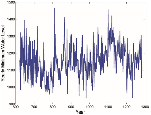
Figure. 1
Fortunately, we can manufacture many more mean-reverting price series than there are traded assets because we can often combine two or more individual price series that are not mean reverting into a portfolio whose net market value (i.e., price) is mean reverting. Those price series that can be combined this way are called cointegrating, and we will describe the statistical tests (CADF test and Johansen test) for cointegration, too. Also, as a by-product of the Johansen test, we can determine the exact weightings of each asset in order to create a mean reverting portfolio. Because of this possibility of artificially creating stationary portfolios, there are numerous opportunities available for mean reversion traders.
As an illustration of how easy it is to profit from mean-reverting price series, I will also describe a simple linear trading strategy, a strategy that is truly “parameter less.”
One clarification: The type of mean reversion we will look at in this chapter may be called time series mean reversion because the prices are supposed to be reverting to a mean determined by its own historical prices. The tests and trading strategies that I depict in this chapter are all tailored to time series mean reversion. There is another kind of mean reversion, called “cross-sectional” mean reversion. Cross-sectional mean reversion means that the cumulative returns of the instruments in a basket will revert to the cumulative return of the basket. This also implies that the short-term relative returns of the instruments are serially anticorrelated. (Relative return of an instrument is the return of that instrument minus the return of the basket.) Since this phenomenon occurs most often for stock baskets, we will discuss how to take advantage of it in next blog when we discuss mean-reverting strategies for stocks and ETFs.
Mean Reversion and Stationarity:
Mean reversion and stationarity are two equivalent ways of looking at the same type of price series, but these two ways give rise to two different statistical tests for such series.
The mathematical description of a mean-reverting price series is that the change of the price series in the next period is proportional to the difference between the mean price and the current price. This gives rise to the ADF test, which tests whether we can reject the null hypothesis that the proportionality constant is zero.
However, the mathematical description of a stationary price series is that the variance of the log of the prices increases slower than that of a geometric random walk. That is, their variance is a sublinear function of time, rather than a linear function, as in the case of a geometric random walk. This sublinear function is usually approximated by τ2H, where τ is the time separating two price measurements, and H is the so-called Hurst exponent, which is less than 0.5 if the price series is indeed stationary (and equal to 0.5 if the price series is a geometric random walk). The Variance Ratio test can be used to see whether we can reject the null hypothesis that the Hurst exponent is actually 0.5.
Note that stationarity is somewhat of a misnomer: It doesn’t mean that the prices are necessarily range bound, with a variance that is independent of time and thus a Hurst exponent of zero. It merely means that the variance increases slower than normal diffusion.
The ADF and Variance Ratio tests are explained mathematically in detail in Walter Beckert’s course notes (Beckert, 2011). Their applications to real-world trading methods are the only thing that interest us here.