Algo Trading Strategy Optimisation

Algo Trading Strategy Optimisation

In prior chapters we have considered how to create both an underlying predictive model (such as with the Suppor Vector Machine and Random Forest Classifier) as well as a trading strategy based upon it. Along the way we have seen that there are many parameters to such models. In the case of an SVM we have the “tuning” parameters γ and C. In a Moving Average Crossover trading strategy we have the parameters for the two lookback windows of the moving average filters.

In this chapter we are going to describe optimisation methods to improve the performance of our trading strategies by tuning the parameters in a systematic fashion. For this we will use mechanisms from the statistical field of Model Selection, such as cross-validation and grid search. The literature on model selection and parameter optimisation is vast and most of the methods are somewhat beyond the scope of this website. I want to introduce the subject here so that you can explore more sophisticated techniques at your own pace.

1.) Parameter Optimisation

At this stage nearly all of the trading strategies and underlying statistical models have required one or more parameters in order to be utilised. In momentum strategies using technical indicators, such as with moving averages (simple or exponential), there is a need to specify a lookback window. The same is true of many mean-reverting strategies, which require a (rolling) lookback window in order to calculate a regression between two time series. Particular statistical machine learning models such as a logistic regression, SVM or Random Forest also require parameters in order to be calculated.

The biggest danger when considering parameter optimisation is that of overfitting a model or trading strategy. This problem occurs when a model is trained on an in sample retained slice of training data and is optimised to perform well (by the appropriate performance measure), but performance degrades substantially when applied to out of sample data. For instance, a trading strategy could perform extremely well in the backtest (the in sample data) but when deployed for live trading can be completely unprofitable.

An additional concern of parameter optimisation is that it can become very computationally expensive. With modern computational systems this is less of an issue than it once was, due to parallelisation and fast CPUs. However, multiple parameter optimisation can increase computational complexity by orders of magnitudes. One must be aware of this as part of the research and development process.

1.1] Which Parameters to Optimise?

A statistical-based algorithmic trading model will often have many parameters and different measures of performance. An underlying statistical learning algorithm will have its own set of parameters. In the case of a multiple linear or logistic regression these would be the β_i coefficients. In the case of a random forest one such parameter would be the number of underlying decision trees to use in the ensemble. Once applied to a trading model other parameters might be entry and exit thresholds, such as a z-score of a particular time series. The z-score itself might have an implicit rolling lookback window. As can be seen the number of parameters can be quite extensive.

In addition to parameters there are numerous means of evaluating the performance of a statistical model and the trading strategy based upon it. We have defined concepts such as the hit rate and the confusion matrix. In addition there are more statistical measures such as the Mean Squared Error (MSE). These are performance measures that would be optimised at the statistical model level, via parameters relevant to their domain.

The actual trading strategy is evaluated on different criteria, such as compound annual growth rate (CAGR) and maximum drawdown. We would need to vary entry and exit criteria, as well as other thresholds that are not directly related to the statistical model. Hence this motivates the question as to which set of parameters to optimise and when.

In the following sections we are going to optimise both the statistical model parameters, at the early research and development stage, as well as the parameters associated with a trading strategy using an underlying optimised statistical model, on each of their respective performance measures.

1.2] Optimisation is Expensive:

With multiple real-valued parameters, optimisation can rapidly become extremely expensive, as each new parameter adds an additional spatial dimension. If we consider the example of a grid search (to be discussed in full below), and have a single parameter α, then we might wish to vary α within the set {0.1,0.2,0.3,0.4,0.5}. This requires 5 simulations.

If we now consider an additional parameter β, which may vary in the range {0.2,0.4,0.6,0.8,1.0}, then we will have to consider 5² = 25 simulations. Another parameter, γ, with 5 variations brings this to 5³ = 125 simulations. If each paramater had 10 separate values to be tested, this would be equal to 10³ = 1000 simulations. As can be seen the parameter search space can rapidly make such simulations extremely expensive.

It is clear that a trade-off exists between conducting an exhaustive parameter search and maintaining a reasonable total simulation time. While parallelism, including many-core CPUs and graphics processing units (GPUs), have mitigated the issue somewhat, we still need to be careful when introducing parameters. This notion of reducing parameters is also an issue of model effectiveness, as we shall see below.

1.3] Overfitting:

Overfitting is the process of optimising a parameter, or set of parameters, against a particular data set such that an appropriate performance measure (or error measure) is found to be maximised (or minimised), but when applied to an unseen data set, such a performance measure degrades substantially. The concept is closely related to the idea of the bias-variance dilemma.

The bias-variance dilemma concerns the situation where a statistical model has a trade-off between being a low-bias model or a low-variance model, or a compromise between the two. Bias refers to the difference between the model’s estimation of a parameter and the true “population” value of the parameter, or erroneous assumptions in the statistical model. Variance refers to the error from the sensitivity of the model to small fluctuations in the training set (in sample data).

In all statistical models one is simultaneously trying to minimise both the bias error and the variance error in order to improve model accuracy. Such a situation can lead to overfitting in models, as the training error can be substantially reduced by introducing models with more flexibility (variation). However, such models can perform extremely poorly on new (out of sample) data since they were essentially “fit” to the in sample data.

A common example of a high-bias, low-variance model is that of linear regression applied to a non-linear data set. Additions of new points do not affect the regression slope dramatically (assuming they are not too far from the remaining data), but since the problem is inherently non-linear, there is a systematic bias in the results by using a linear model.

A common example of a low-bias, high-variance model is that of a polynomial spline fit applied to a non-linear data set. The parameter of the model (the degree of the polynomial) could be adjusted to fit such a model very precisely (i.e. low-bias on the training data), but additions of new points would almost certainly lead to the model having to modify its degree of polynomial to fit the new data. This would make it a very high-variance model on the in sample data. Such a model would likely have very poor predictability or inferential capability on out of sample data.

Overfitting can also manifest itself on the trading strategy and not just the statistical model. For instance, we could optimise the Sharpe ratio by varying entry and exit threshold parameters. While this may improve profitability in the backtest (or minimise risk substantially), it would likely not be behaviour that is replicated when the strategy was deployed live, as we might have been fitting such optimisations to noise in the historical data.

We will discuss techniques below to minimise overfitting, as much as possible. However one has to be aware that it is an ever-present danger in both algorithmic trading and statistical analysis in general.

2.) Model Selection

In this section we are going to consider how to optimise the statistical model that will underly a trading strategy. In the field of statistics and machine learning this is known as Model Selection. While I won’t present an exhaustive discussion on the various model selection techniques, I will describe some of the basic mechanisms such as Cross Validation and Grid Search that work well for trading strategies.

2.1] Cross Validation:

Cross Validation is a technique used to assess how a statistical model will generalise to new data that it has not been exposed to before. Such a technique is usually used on predictive models, such as the aforementioned supervised classifiers used to predict the sign of the following daily returns of an asset price series. Fundamentally, the goal of cross validation is to minimise error on out of sample data without leading to an overfit model.

In this section we will describe the training/test split and k-fold cross validation, as well as use techniques within Scikit-Learn to automatically carry out these procedures on statistical models we have already developed.

Train/Test Split

The simplest example of cross validation is known as a training/test split, or a 2-fold cross validation. Once a prior historical data set is assembled (such as a daily time series of asset prices), it is split into two components. The ratio of the split is usually varied between 0.5 and 0.8. In the latter case this means 80% of the data is used for training and 20% is used for testing. All of the statistics of interest, such as the hit rate, confusion matrix or mean-squared error are calculated on the test set, which has not been used within the training process.

To carry out this process in Python with Scikit-Learn we can use the sklearncross^_validation train_test_split method. We will continue with our model as discussed in the chapter on Forecasting. In particular, we are going to modify forecast.py and create a new file called train^_test^_split.py. We will need to add the new import to the list of imports:

In forecast.py we originally split the data based on a particular date within the time series:

This can be replaced with the method train^_test^_split from Scikit-Learn in the train^_test^_split.py file. For completeness, the full __main__ method is provided below:

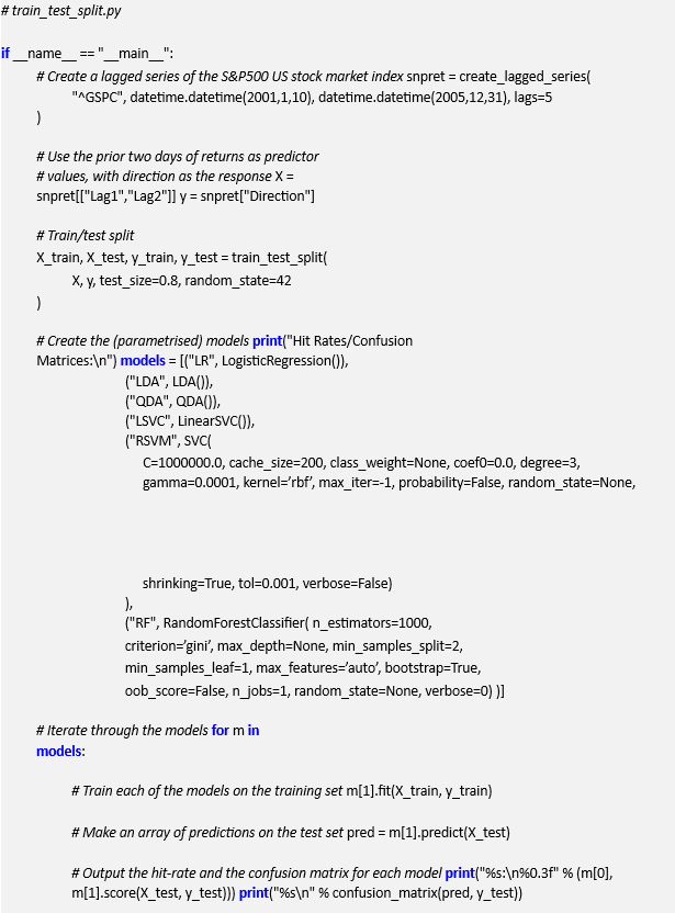
Notice that we have picked the ratio of the training set to be 80% of the data, leaving the testing data with only 20%. In addition we have specified a random_state to randomise the sampling within the selection of data. This means that the data is not sequentially divided chronologically, but rather is sampled randomly.

The results of the cross-validation on the model are as follows (yous will likely appear slightly different due to the nature of the fitting procedure):

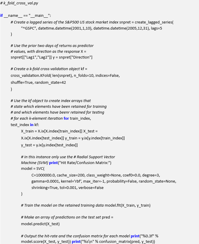
Hit Rates/Confusion Matrices:

It can be seen that the hit rates are substantially lower than those found in the aforementioned forecasting chapter. Consequently we can likely conclude that the particular choice of training/test split lead to an over-optimistic view of the predictive capability of the classifier.

The next step is to increase the number of times a cross-validation is performed in order to minimise any potential overfitting. For this we will use k-fold cross validation.

K-Fold Cross Validation

Rather than partitioning the set into a single training and test set, we can use k-fold cross validation to randomly partition the the set into k equally sized subsamples. For each iteration (of which there are k), one of the k subsamples is retained as a test set, while the remaining k −1 subsamples together form a training set. A statistical model is then trained on each of the k folds and its performance evaluated on its specific k-th test set.

The purpose of this is to combine the results of each model into an emsemble by means of averaging the results of the prediction (or otherwise) to produce a single prediction. The main benefit of using k-fold cross validation is that the every predictor within the original data set is used both for training and testing only once.

This motivates a question as to how to choose k, which is now another parameter! Generally, k = 10 is used but one can also perform another analysis to choose an optimal value of k.

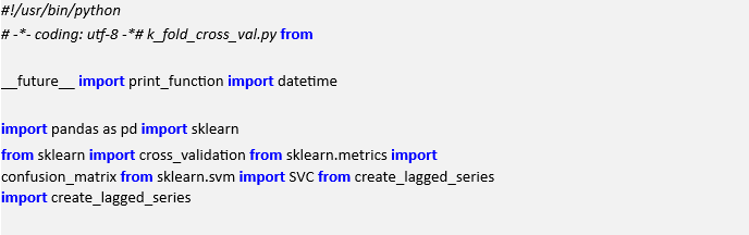
We will now make use of the cross^_validation module of Scikit-Learn to obtain the KFold k-fold cross validation object. We create a new file called k^_fold^_cross^_val.py, which is a copy of train^_test^_split.py and modify the imports by adding the following line:

We then need to make changes the ^__main^__ function by removing the train^_test^_split method and replacing it with an instance of KFold. It takes five parameters.

The first isthe length of the dataset, which in this case 1250 days. The second value is K representing the number of folds, which in this case is 10. The third value is indices, which I have set to False. This means that the actual index values are used for the arrays returned by the iterator. The fourth and fifth are used to randomise the order of the samples.

As before in forecast.py and train^_test^_split.py we obtain the lagged series of the S&P500. We then create a set of vectors of predictors (X) and responses (y). We then utilise the KFold object and iterate over it. During each iteration we create the training and testing sets for each of the X and y vectors. These are then fed into a radial support vector machine with identical parameters to the aforementioned files and the model is fit.

Finally the hit rate and confusion matrix for each instance of the SVM is output.

The output of the code is as follows:

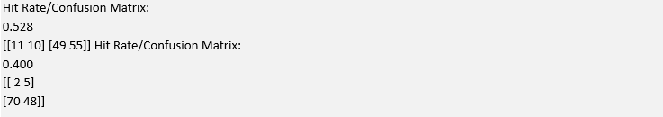
It is the clear that the hit rate and confusion matrices vary dramatically across the various folds. This is indicative that the model is prone to overfitting, on this particular dataset. A remedy for this is to use significantly more data, either at a higher frequency or over a longer duration.

In order to utilise this model in a trading strrategy it would be necessary to combine each of these individually trained classifiers (i.e. each of the K objects) into an ensemble average and then use that combined model for classification within the strategy.

Note that technically it is not appropriate to use simple cross-validation techniques on temporally ordered data (i.e. time-series). There are more sophisticated mechanisms for coping with autocorrelation in this fashion, but I wanted to highlight the approach so we have used time series data for simplicity.

2.2] Grid Search:

We have so far seen that k-fold cross validation helps us to avoid overfitting in the data by performing validation on every element of the sample. We now turn our attention to optimising the hyper-parameters of a particular statistical model. Such parameters are those not directly learnt by the model estimation procedure. For instance, C and γ for a support vector machine. In essence they are the parameters that we need to specify when calling the initialisation of each statistical model. For this procedure we will use a process known as a grid search.

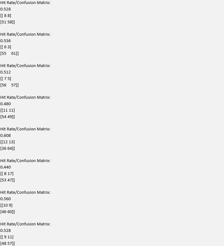
The basic idea is to take a range of parameters and assess the performance of the statistical model on each parameter element within the range. To achieve this in Scikit-Learn we can create a ParameterGrid. Such an object will produce a list of Python dictionaries that each contain a parameter combination to be fed into a statistical model.

An example code snippet that produces a parameter grid, for parameters related to a support vector machine, is given below:

Now that we have a suitable means of generating a ParameterGrid we need to feed this into a statistical model iteratively to search for an optimal performance score. In this case we are going to seek to maximise the hit rate of the classifier.

The GridSearchCV mechanism from Scikit-Learn allows us to perform the actual grid search. In fact, it allows us to perform not only a standard grid search but also a cross validation scheme at the same time.

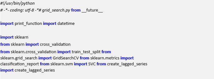
We are now going to create a new file, grid^_search.py, that once again uses create^_lagged^_series.py and a support vector machine to perform a cross-validated hyperparameter grid search. To this end we must import the correct libraries:

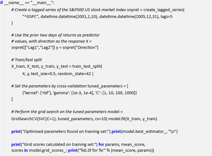
As before with k^_fold^_cross^_val.py we create a lagged series and then use the previous two days of returns as predictors. We initially create a training/test split such that 50% of the data can be used for training and cross validation while the remaining data can be “held out” for evaluation.

Subsequently we create the tuned_parameters list, which contains a single dictionary denoting the parameters we wish to test over. This will create a cartesian product of all parameter lists, i.e. a list of pairs of every possible parameter combination.

Once the parameter list is created we pass it to the GridSearchCV class, along with the type of classifier that we’re interested in (namely a radial support vector machine), with a k-fold cross-validation k-value of 10.

Finally, we train the model and output the best estimator and its associated hit rate scores. In this way we have not only optimised the model parameters via cross validation but we have also optimised the hyperparameters of the model via a parametrised grid search, all in one class! Such succinctness of the code allows significant experimentation without being bogged down by excessive “data wrangling”.

The output of the grid search cross validation procedure is as follows:

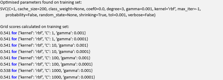
As we can see γ = 0.001 and C = 1 provides the best hit rate, on the validation set, for this particular radial kernel support vector machine. This model could now form the basis of a forecasting-based trading strategy, as we have previously demonstrated in the prior chapter.

3.) Optimising Strategies

Up until this point we have concentrated on model selection and optimising the underlying statistical model that (might) form the basis of a trading strategy. However, a predictive model and a functioning, profitable algorithmic strategy are two different entities. We now turn our attention to optimising parameters that have a direct effect on profitability and risk metrics.

To achieve this we are going to make use of the event-driven backtesting software that was described in a previous chapter. We will consider a particular strategy that has three parameters associated with it and search through the space formed by the cartesian product of parameters, using a grid search mechanism. We will then attempt to maximise particular metrics such as the Sharpe Ratio or minimise others such as the maximum drawdown.

3.1] Intraday Mean Reverting Pairs:

The strategy of interest to us in this chapter is the “Intraday Mean Reverting Equity Pairs Trade” using the energy equities AREX and WLL. It contains three parameters that we are capable of optimising: The linear regression lookback period, the residuals z-score entry threshold and the residuals z-score exit threshold.

We will consider a range of values for each parameter and then calculate a backtest for the strategy across each of these ranges, outputting the total return, Sharpe ratio and drawdown characteristics of each simulation, to a CSV file for each parameter set. This will allow us to ascertain an optimised Sharpe or minimised max drawdown for our trading strategy.

3.2] Parameter Adjustment:

Since the event-driven backtesting software is quite CPU-intensive, we will restrict the parameter range to three values per parameter. This will give us a total of 3³ = 27 separate simulations to carry out. The parameter ranges are listed below:

• OLS Lookback Window – w_l ∈ {50,100,200}
• Z-Score Entry Threshold – z_h ∈ {2.0,3.0,4.0}
• Z-Score Exit Threshold – z_l ∈ {0.5,1.0,1.5}

To carry out the set of simulations a cartesian product of all three ranges will be calculated and then the simulation will be carried out for each combination of parameters.

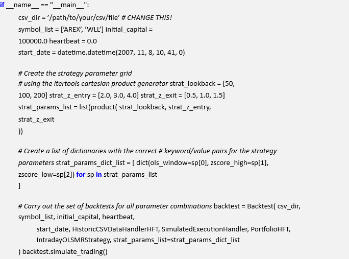
The first task is to modify the intraday^_mr.py file to include the product method from the itertools library:

We can then modify the __main__ method to include the generation of a parameter list for all three of the parameters discussed above.

The first task is to create the actual paramater ranges for the OLS lookback window, the zscore entry threshold and the zscore exit threshold. Each of these has three separate variations leading to a total of 27 simulations.

Once the ranges are created the itertools.product method is used to create a cartesian product of all variations, which is then fed into a list of dictionaries to ensure that the correct keyword arguments are passed to the Strategy object.

Finally the backtest is instantiated with the strat_params_list forming the final keyword argument:

The next step is to modify the Backtest object in backtest.py to be able to handle multiple parameter sets. We need to modify the ^_generate^_trading^_instances method to have an argument that represents the particular parameter set on creation of a new Strategy object:

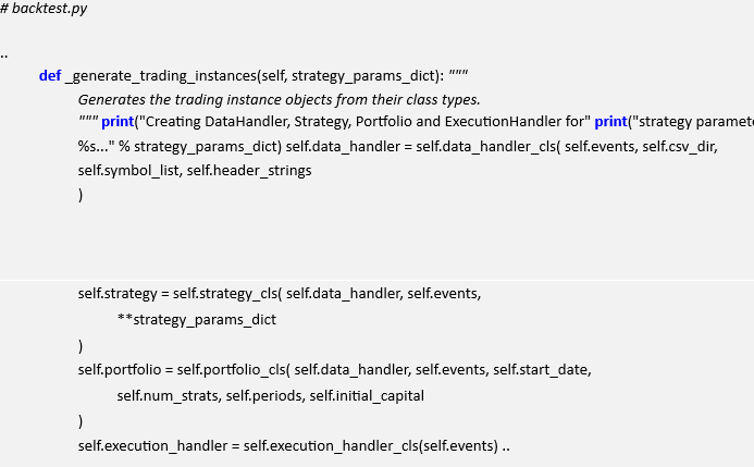
This method is now called within a strategy parameter list loop, rather than at construction of the Backtest object. While it may seem wasteful to recreate all of the data handlers, event queues and portfolio objects for each parameter set, it ensures that all of the iterators have been reset and that we are truly starting with a “clean slate” for each simulation.

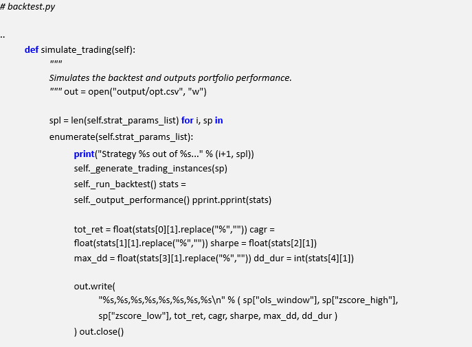
The next task is to modify the simulate_trading method to loop over all variants of strategy parameters. The method creates an output CSV file that is used to store parameter combinations and their particular performance metrics. This will allow us later to plot performance characteristics across parameters.

The method loops over all of the strategy parameters and generates a new trading instance on every simulation. The backtest is then executed and the statistics calculated. These are stored and output into the CSV file. Once the simulation ends, the output file is closed:

On my desktop system, this process takes some time! 27 parameter simulations across more than 600,000 data points per simulation takes around 3 hours. The backtester has not been parallelised at this stage, so concurrent running of simulation jobs would make the process a lot faster. The output of the current parameter study is given below. The columns are given by OLS Lookback, ZScore High, ZScore Low, Total Return (%), CAGR (%), Sharpe, Max DD (%), DD Duration (minutes):

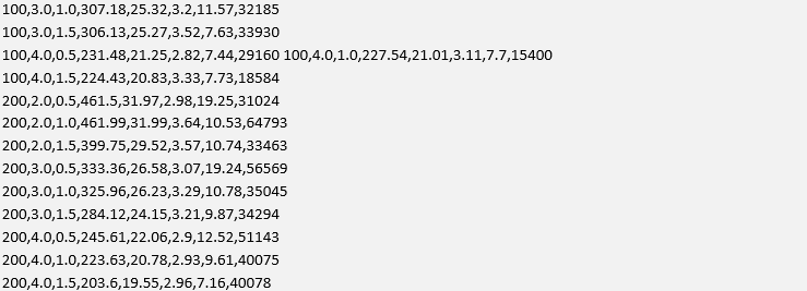
We can see that for this particular study the parameter values of w_l = 50, z_h = 3.0 and z_l = 1.5 provide the best Sharpe ratio at S = 3.71. For this Sharpe ratio we have a total return of 294.91% and a maximum drawdown of 8.04%. The best total return of 461.99%, albeit with a maximum drawdown of 10.53% is given by the parameter set of w_l = 200, z_h = 2.0 and z_l = 1.0.

3.3] Visualisation:

As a final task in strategy optimisation, we are now going to visualise the performance characteristics of the backtester using Matplotlib, which is an extremely useful step when carrying out initial strategy research. Unfortunately we are the situation where we have a three-dimensional problem and so performance visualisation is not straightforward! However, there are some partial remedies to the situation.

Firstly, we could fix the value of one parameter and take a “parameter slice” through the remainder of the “data cube”. For instance we could fix the lookback window to be 100 and then see who the variation in z-score entry and exit thresholds affects the Sharpe Ratio or the maximum drawdown.

To achieve this we will use Matplotlib. We will read the output CSV and reshape the data such that we can visualise the results.

Sharpe/Drawdown Heatmap

We will fix the lookback period of w_l = 100 and then generate a 3 × 3 grid and “heatmap” of the Sharpe ratio and maximum drawdown for the variation in z-score thresholds.

In the following code we import the output CSV file. The first task is to filter out the lookback periods that are not of interest (w_l ∈ {50,200}). Then we reshape the remaining performance data into two 3 × 3 matrices. The first represents the Sharpe ratio for each z-score threshold combination while the second represents maximum drawdown.

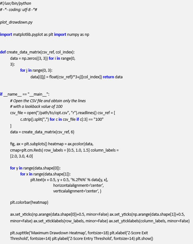
Here is the code for creating the Sharpe Ratio heatmap. We first import Matplotlib and

NumPy. Then we define a function called create_data_matrix which reshapes the Sharpe Ratio data into a 3 × 3 grid. Within the __main__ function we open the CSV file (make sure to change the path on your system!) and exclude any lines not referencing a lookback period of 100.

We then create a blue-shaded heatmap and apply the correct row/column labels using the z-score thresholds. Subsequently we place the actual value of the Sharpe Ratio onto the heatmap.

Finally, we set the ticks, labels, title and then plot the heatmap:

plt.ylabel(’Z-Score Entry Threshold’, fontsize=14) plt.show()

The plot for the maximum drawdown is almost identical with the exception that we use a red-shaded heatmap and alter the column index in the create_data_matrix function to use the maximum drawdown percentage data.

The heatmaps produced from the above snippets are given in Fig.3.3:

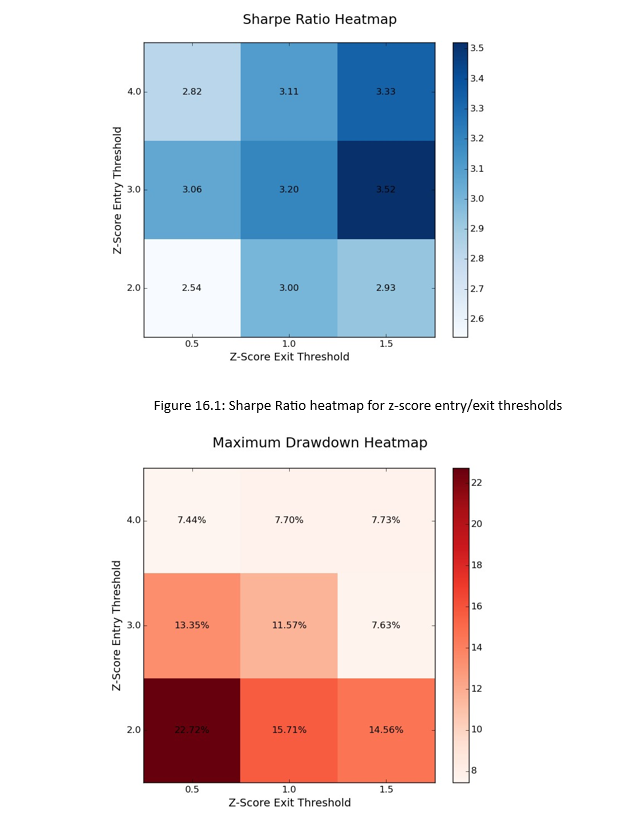
Figure .2: Maximum Drawdown heatmap for z-score entry/exit thresholds

At w_l = 100 the differences betwee the smallest and largest Sharpe Ratios, as well as the smallest and largest maximum drawdowns, is readily apparent. The Sharpe Ratio is optimised for larger entry and exit thresholds, while the drawdown is minimised in the same region. The Sharpe Ratio and maximum drawdown are at their worst when both the entry and exit thresholds are low.

This clearly motivates us to consider using relatively high entry and exit thresholds for this strategy when deployed into live trading.

Read Also; Algo Trading Strategy Implementation