Processing Financial Data
The discussion will begin with an overview of the different types of data that will be of interest to algorithmic traders. The frequency of the data will then be considered, from quarterly data (such as SEC reports) through to tick and order book data on the millisecond scale. Sources of such data (both free and commercial) will then be outlined along with code for obtaining the data. Finally, cleansing and preparation of the data for usage in strategies will be discussed.
1.) Market and Instrument Classification
As algorithmic traders we are often interested in a broad range of financial markets data. This can range from underlying and derivative instrument time series prices, unstructured text-based data (such as news articles) through to corporate earnings information. In this will predominantly discuss financial time series data.
1.1] Markets:
US and international equities, foreign exchange, commodities and fixed income are the primary sources of market data that will be of interest to an algorithmic trader. In the equities market it is still extremely common to purchase the underlying asset directly, while in the latter three markets highly liquid derivative instruments (futures, options or more exotic instruments) are more commonly used for trading purposes.
This broad categorisation essentially makes it relatively straightforward to deal in the equity markets, albeit with issues surrounding data handling of corporate actions (see below). Thus a large part of the retail algorithmic trading landscape will be based around equities, such as direct corporate shares or Exchange Traded Funds (ETFs). Foreign exchange (“forex”) markets are also highly popular since brokers will allow margin trading on percentage in point (PIP) movements. A pip is one unit of the fourth decimal point in a currency rate. For currencies denominated in US dollars this is equivalent to 1/100th of a cent.
Commodities and fixed income markets are harder to trade in the underlying directly. A retail algorithmic trader is often not interested in delivering barrels of oil to an oil depot! Instead, futures contracts on the underlying asset are used for speculative purposes. Once again, margin trading is employed allowing extensive leverage on such contracts.
1.2] Instruments:
A wide range of underlying and derivative instruments are available to the algorithmic trader. The following table describes the common use cases of interest.
| Market | Instruments |
| Equities/Indices | Stock, ETFs, Futures, Options |
| Foreign Exchange | Margin/Spot, ETFs, Futures, Options |
| Commodities | Futures, Options |
| Fixed Income | Futures, Options |
For the purposes of this book we will concentrate almost exclusively upon equities and ETFs to simplify the implementation.
1.3] Fundamental Data:
Although algorithmic traders primarily carry out analysis of financial price time series, fundamental data (of varying frequencies) is also often added to the analysis. So-called Quantitative Value (QV) strategies rely heavily on the accumulation and analysis of fundamental data, such as macroeconomic information, corporate earnings histories, inflation indexes, payroll reports, interest rates and SEC filings. Such data is often also in temporal format, albeit on much larger timescales over months, quarters or years. QV strategies also operate on these timeframes.
1.4] Unstructured Data:
Unstructured data consists of documents such as news articles, blog posts, papers or reports. Analysis of such data can be complicated as it relies on Natural Language Processing (NLP) techniques. One such use of analysing unstructured data is in trying to determine the sentiment context. This can be useful in driving a trading strategy. For instance, by classifying texts as “bullish”, “bearish” or “neutral” a set of trading signals could be generated. The term for this process is sentiment analysis.
Python provides an extremely comprehensive library for the analysis of text data known as the Natural Language Toolkit (NLTK). Indeed an O’Reilly book on NLTK can be downloaded for free via the authors’ website – Natural Language Processing with Python[3].
Full-Text Data
There are numerous sources of full-text data that may be useful for generating a trading strategy. Popular financial sources such as Bloomberg and the Financial Times, as well as financial commentary blogs such as Seeking Alpha and ZeroHedge, provide significant sources of text to analyse. In addition, proprietary news feeds as provided by data vendors are also good sources of such data.
In order to obtain data on a larger scale, one must make use of “web scraping” tools, which are designed to automate the downloading of websites en-masse. Be careful here as automated web-scraping tools sometimes breach the Terms Of Service for these sites. Make sure to check before you begin downloading this sort of data. A particularly useful tool for web scraping, which makes the process efficient and structured, is the ScraPy library.
Social Media Data
In the last few years there has been significant interest in obtaining sentiment information from social media data, particularly via the Twitter micro-blogging service. Back in 2011, a hedge fund was launched around Twitter sentiment, known as Derwent Capital. Indeed, academic studies[4] have shown evidence that it is possible to generate a degree of predictive capability based on such sentiment analysis.
2.) Frequency of Data
Frequency of data is one of the most important considerations when designing an algorithmic trading system. It will impact every design decision regarding the storage of data, backtesting a strategy and executing an algorithm.
Higher frequency strategies are likely to lead to more statistically robust analysis, simply due to the greater number of data points (and thus trades) that will be used. HFT strategies often require a significant investment of time and capital for development of the necessary software to carry them out.
Lower frequency strategies are easier to develop and deploy, since they require less automation. However, they will often generate far less trades than a higher-frequency strategy leading to a less statistically robust analysis.
2.1] Weekly and Monthly Data:
Fundamental data is often reported on a weekly, monthly, quarterly or even yearly basis. Such data include payroll data, hedge fund performance reports, SEC filings, inflation-based indices (such as the Consumer Price Index, CPI), economic growth and corporate accounts.
Storage of such data is often suited to unstructured databases, such as MongoDB, which can handle hierarchically-nested data and thus allowing a reasonable degree of querying capability. The alternative is to store flat-file text in a RDBMS, which is less appropriate, since full-text querying is trickier.
2.2] Daily Data:
The majority of retail algorithmic traders make use of daily (“end of day”/EOD) financial time series data, particularly in equities and foreign exchange. Such data is freely available (see below), but often of questionable quality and subject to certain biases. End-of-day data is often stored in RDBMS, since the nature of ticker/symbol mapping naturally applies to the relational model.
EOD data does not entail particularly large storage requirements. There are 252 trading days in a year for US exchanges and thus for a decade there will be 2,520 bars per security. Even with a universe of 10,000 symbols this is 25,200,000 bars, which can easily be handled within a relational database environment.
2.3] Intraday Bars:
Intraday strategies often make use of hourly, fifteen-, five-, one-minutely or secondly OHLCV bars. Intraday feed providers such as QuantQuote and DTN IQFeed will often provide minutely or secondly bars based on their tick data.
Data at such frequencies will possess many “missing” bars simply because no trades were carried out in that time period. Pandas can be used to pad these values forward, albeit with a decrease in data accuracy. In addition pandas can also be used to create data on less granular timescales if necessary.
For a ten year period, minutely data will generate almost one million bars per security. Similarly for secondly data the number of data points over the same period will total almost sixty million per security. Thus to store one thousand of such securities will lead to sixty billion bars of data. This is a large amount of data to be kept in an RDBMS and consequently more sophisticated approaches are required.
2.4] Tick and Order Book Data:
When a trade is filled at an exchange, or other venue, a tick is generated. Tick feeds consist of all such transactions per exchange. Retail tick feeds are stored with each datum having a timestamp accurate to the millisecond level. Tick data often also includes the updated best bid/ask price. The storage of tick data is well beyond the scope of this book but needless to say the volumes of such data are substantial. Common storage mechanisms include HDF5, kdb and simply flat-file/CSV.
Multiple limit orders at an exchange lead to the concept of an order book. This is essentially the list of all bid and ask limit orders at certain volumes for each market participant. It leads to the definition of the bid-ask spread (or simply the “spread”), which is the smallest difference in the bid and ask prices for the “top of book” orders. Creating a historical representation, or a market simulator, of a limit order book is usually necessary for carrying out ultra high frequency trading (UHFT) strategies. The storage of such data is complex and as such will be outside the scope of this book.
3.) Sources of Data
There are numerous sources and vendors of financial data. They vary substantially in breadth, timeliness, quality and price.
Broadly speaking, financial market data provided on a delayed daily frequency or longer is available freely, albeit with dubious overall quality and the potential for survivorship bias. To obtain intraday data it is usually necessary to purchase a commercial data feed. The vendors of such feeds vary tremendously in their customer service capability, overall feed quality and breadth of instruments.
3.1] Free Sources:
Free end-of-day bar data, which consists of Open-High-Low-Close-Volume (OHLCV) prices for instruments, is available for a wide range of US and international equities and futures from Yahoo Finance, Google Finance and Quandl.
Yahoo Finance
Yahoo Finance is the “go to” resource when forming an end-of-day US equities database. The breadth of data is extremely comprehensive, listing thousands of traded equities. In addition stock-splits and dividends are handled using a back-adjustment method, arising as the “Adj Close” column in the CSV output from the API (which we discuss below). Thus the data allows algorithmic traders to get started rapidly and for zero cost.
I have personally had a lot of experience in cleaning Yahoo data. I have to remark that the data can be quite erroneous. Firstly, it is subject to a problem known as backfilling. This problem occurs when past historical data is corrected at a future date, leading to poor quality backtests that change as your own database is re-updated. To handle this problem, a logging record is usually added to the securities master (in an appropriate logging table) whenever a historical data point is modified.
Secondly, the Yahoo feed only aggregates prices from a few sources to form the OHLCV points. This means that values around the open, high, low and close can be deceptive, as other exchanges/liquidity sources may have executed differing prices in excess of the values.
Thirdly, I have noticed that when obtaining financial data en-masse from Yahoo, that errors do creep into the API. For instance, multiple calls to the API with identical date/ticker parameters occasionally lead to differing result sets. This is clearly a substantial problem and must be carefully checked for.
In summary be prepared to carry out some extensive data cleansing on Yahoo Finance data, if you choose to use it to populate a large securities master, and need highly accurate data.
Quandl
Quandl is a relatively new service which purports to be “The easiest way to find and use numerical data on the web”. I believe they are well on the way to achieving that goal! The service provides a substantial daily data set of US and international equities, interest rates, commodities/futures, foreign exchange and other economic data. In addition, the database is continually expanded and the project is very actively maintained.
All of the data can be accessed by a very modern HTTP API (CSV, JSON, XML or HTML), with plugins for a wide variety of programming languages including R, Python, Matlab, Excel, Stata, Maple, C#, EViews, Java, C/C++, .NET, Clojure and Julia. Without an account 50 calls to the API are allowed per day, but this can be increased to 500 if registering an account. In fact, calls can be updated to 5,000 per hour if so desired by contacting the team.
I have not had a great deal of experience with Quandl “at scale” and so I can’t comment on the level of errors within the dataset, but my feeling is that any errors are likely to be constantly reported and corrected. Thus they are worth considering as a primary data source for an end-of-day securities master.
Later in the chapter we will discuss how to obtain US Commodities Futures data from Quandl with Python and pandas.
3.2] Commercial Sources:
In order to carry out intraday algorithmic trading it is usually necessary to purchase a commercial feed. Pricing can range anywhere from $30 per month to around $500 per month for “retail level” feeds. Institutional quality feeds will often be in the low-to-mid four figure range per month and as such I won’t discuss them here.
EODData
I have utilised EODData in a fund context, albeit only with daily data and predominantly for foreign exchange. Despite their name they do provide a degree of intraday sources. The cost is $25 per month for their “platinum” package.
The resource is very useful for finding a full list of traded symbols on global exchanges, but remember that this will be subject to survivorship bias as I believe the list represents current listed entities.
Unfortunately (at least back in 2010) I found that the stock split feed was somewhat inaccurate (at least when compared to Morningstar information). This lead to some substantial spike issues (see below) in the data, which increased friction in the data cleansing process.
DTN IQFeed
DTN IQFeed are one of the most popular data feeds for the high-end retail algorithmic trader. They claim to have over 80,000 customers. They provide real-time tick-by-tick data unfiltered from the exchange as well as a large quantity of historic data.
The pricing starts at $50 per month, but in reality will be in the $150-$200 per month range once particular services are selected and exchange fees are factored in. I utilise DTN IQFeed for all of my intraday equities and futures strategies. In terms of historical data, IQFeed provide for equities, futures and options:
- 180 calendar days of tick (every trade)
- 7+ years of 1 minute historical bars
- 15+ years of daily historical bars
The major disadvantage is that the DTN IQFeed software (the mini-server, not the charting tools) will only run on Windows. This may not be a problem if all of your algorithmic trading is carried out in this operating system, but I personally develop all my strategies in Ubuntu Linux. However, although I have not actively tested it, I have heard it is possible to run DTN IQFeed under the WINE emulator.
Below we will discuss how to obtain data from IQFeed using Python in Windows.
QuantQuote
QuantQuote provide reasonably priced historical minute-, second- and tick-level data for US equities going back to 1998. In addition they provide institutional level real-time tick feeds, although this is of less interest to retail algorithmic traders. One of the main benefits of QuantQuote is that their data is provided free of survivorship bias, due to their TickMap symbol-matching software and inclusion of all stocks within a certain index through time.
As an example, to purchase the entire history of the S&P500 going back to 1998 in minutelybars, inclusive of de-listed stocks, the cost at the time of writing was $895. The pricing scales with increasing frequency of data.
QuantQuote is currently the primary provider of market data to the QuantConnect webbased backtesting service. QuantQuote go to great lengths to ensure minimisation of error, so if you are looking for a US equities only feed at high resolution, then you should consider using their service.
4.) Obtaining Data
In this section we are going to discuss how to use Quandl, pandas and DTN IQFeed to download financial market data across a range of markets and timeframes.
4.1] Yahoo Finance and Pandas:
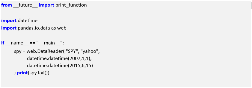
The pandas library makes it exceedingly simple to download EOD data from Yahoo Finance. Pandas ships with a DataReader component that ties into Yahoo Finance (among other sources). Specifying a symbol with a start and end date is sufficient to download an EOD series into a pandas DataFrame, which allows rapid vectorised operations to be carried out:
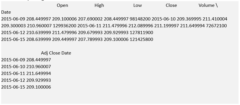
The output is given below:
Note that in pandas 0.17.0, pandas.io.data will be replaced by a separate pandas-datareader package. However, for the time being (i.e. pandas versions 0.16.x) the syntax to import the data reader is import pandas.io.data as web.
In the next section we will use Quandl to create a more comprehensive, permanent download solution
4.2] Quandl and Pandas:
Up until recently it was rather difficult and expensive to obtain consistent futures data across exchanges in frequently updated manner. However, the release of the Quandl service has changed the situation dramatically, with financial data in some cases going back to the 1950s. In this section we will use Quandl to download a set of end-of-day futures contracts across multiple delivery dates.
Signing Up For Quandl
The first thing to do is sign up to Quandl. This will increase the daily allowance of calls to their API. Sign-up grants 500 calls per day, rather than the default 50. Visit the site at www.quandl.com:
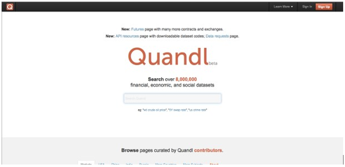
Figure 1: The Quandl homepage
Click on the sign-up button on the top right:
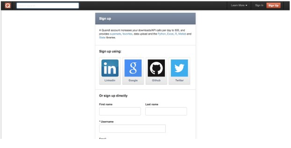
Figure 2: The Quandl sign-up page
Once you’re signed in you’ll be returned to the home page:
Figure 3: The Quandl authorised home page
Quandl Futures Data
Now click on the “New: Futures page…” link to get to the futures homepage:
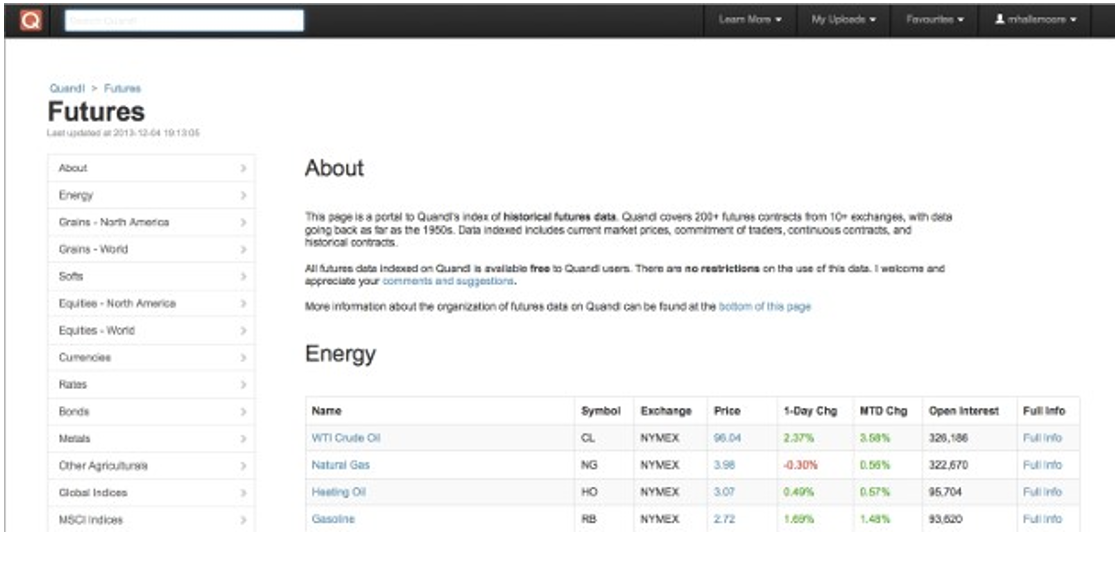
Figure 4: The Quandl futures contracts home page
For this tutorial we will be considering the highly liquid E-Mini S&P500 futures contract, which has the futures symbol ES. To download other contracts the remainder of this tutorial can be carried out with additional symbols replacing the reference to ES.
Click on the E-Mini S&P500 link (or your chosen futures symbol) and you’ll be taken to the following screen:
Scrolling further down the screen displays the list of historical contracts going back to 1997:
Click on one of the individual contracts. As an example, I have chosen ESZ2014, which refers to the contract for December 2014 ’delivery’. This will display a chart of the data:
By clicking on the “Download” button the data can be obtained in multiple formats: HTML, CSV, JSON or XML. In addition we can download the data directly into a pandas DataFrame using the Python bindings. While the latter is useful for quick “prototyping” and exploration of the data, in this section we are considering the development of a longer term data store. Click the download button, select “CSV” and then copy and paste the API call: The API call will have the following form:
( http://www.quandl.com/api/v1/datasets/OFDP/FUTURE_ESZ2014.csv?&auth_token=MY_AUTH_TOKEN&trim_start=2013-09-18&trim_end=2013-12-04&sort_order=desc )
The authorisation token has been redacted and replaced with MY_AUTH_TOKEN. It will be necessary to copy the alphanumeric string between “auth_token=” and “&trim_start” for;
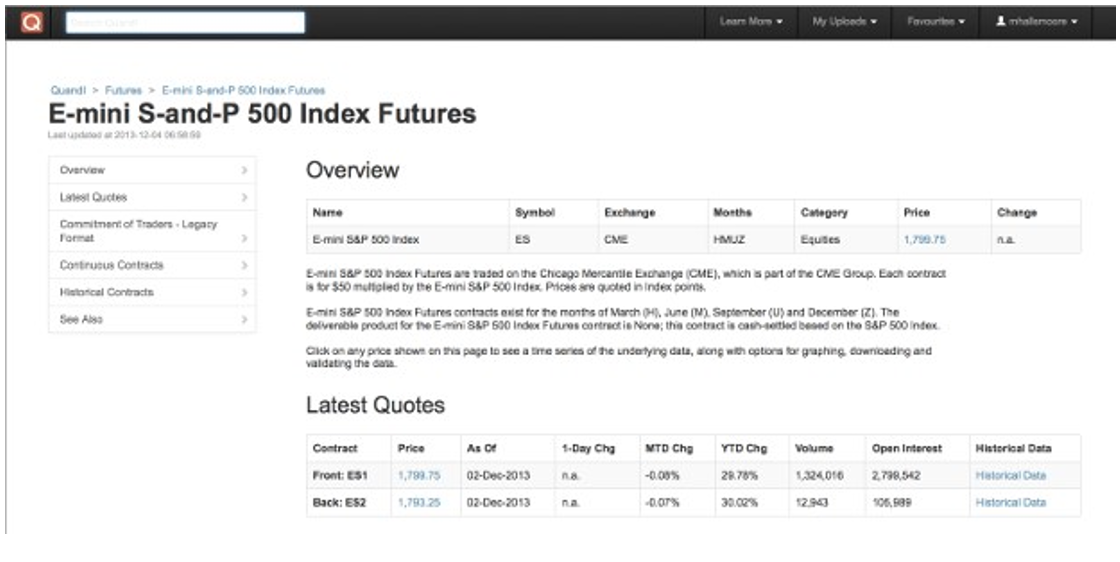
Figure 5: E-Mini S&P500 contract page
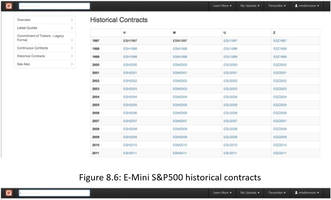
Figure 6: E-Mini S&P500 historical contracts
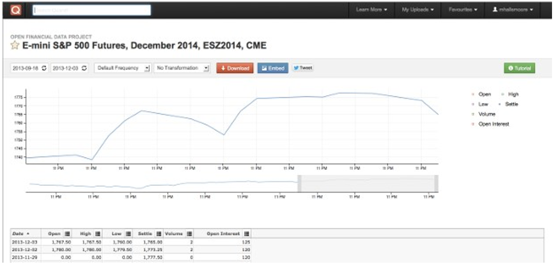
Figure 7: Chart of ESZ2014 (December 2014 delivery)
later usage in the Python script below. Do not share it with anyone as it is your unique authorisation token for Quandl downloads and is used to determine your download rate for the day.
This API call will form the basis of an automated script which we will write below to download a subset of the entire historical futures contract.
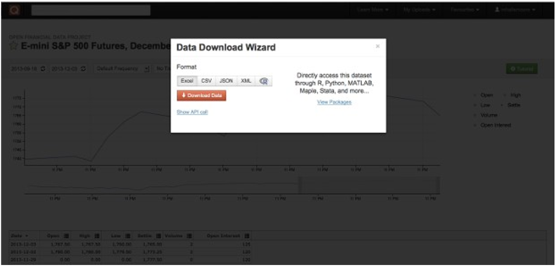
Figure 8: Download modal for ESZ2014 CSV file
Downloading Quandl Futures into Python
Because we are interested in using the futures data long-term as part of a wider securities master database strategy we want to store the futures data to disk. Thus we need to create a directory to hold our E-Mini contract CSV files. In Mac/Linux (within the terminal/console) this is achieved by the following command:
( cd /PATH/TO/YOUR/quandl_data.py mkdir -p quandl/futures/ES )
Note: Replace /PATH/TO/YOUR above with the directory where your quandl_data.py file is located.
This creates a subdirectory of called quandl, which contains two further subdirectories for futures and for the ES contracts in particular. This will help us to organise our downloads in an ongoing fashion.
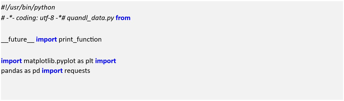
In order to carry out the download using Python we will need to import some libraries. In particular we will need requests for the download and pandas and matplotlib for plotting and data manipulation:
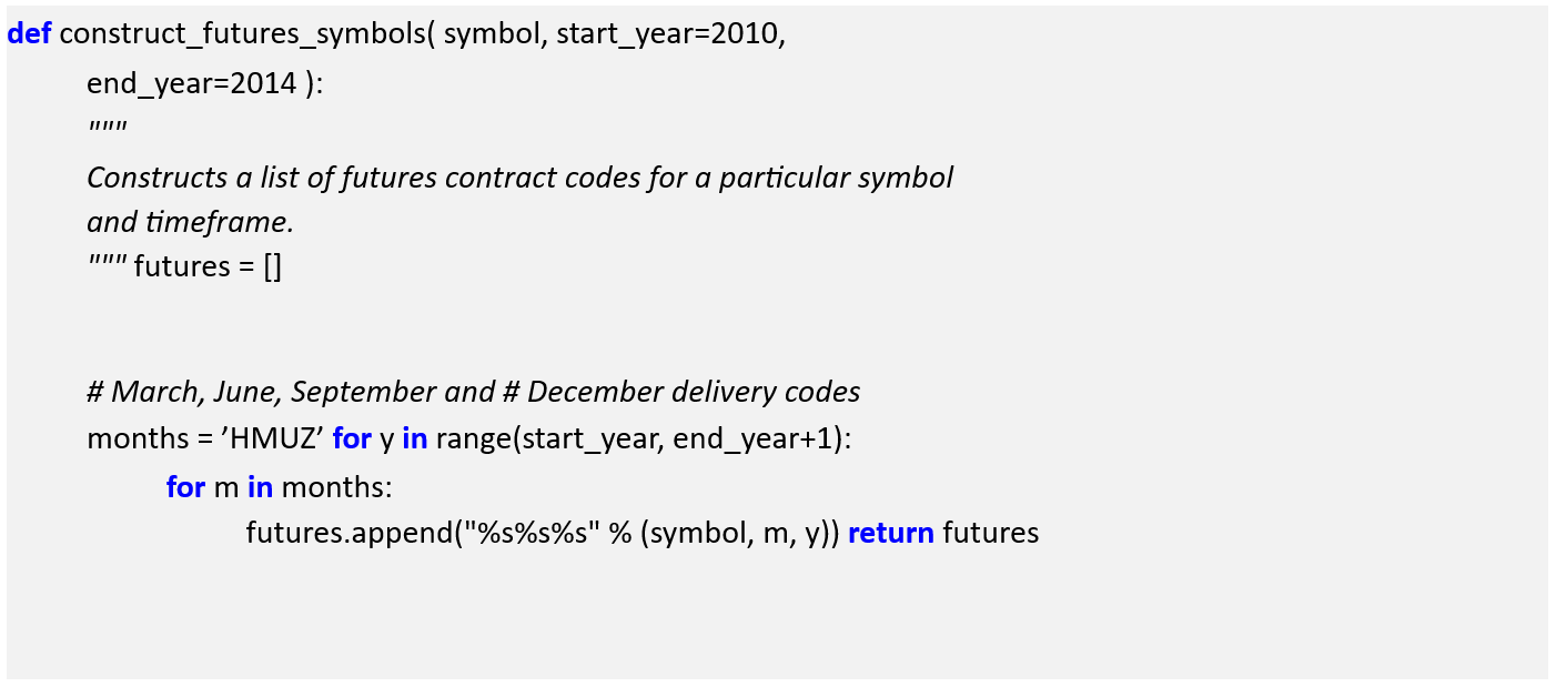
The first function within the code will generate the list of futures symbols we wish to download. I’ve added keyword parameters for the start and end years, setting them to reasonable values of 2010 and 2014. You can, of course, choose to use other timeframes:
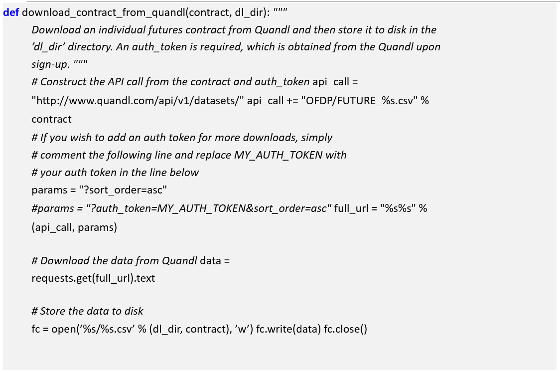
Now we need to loop through each symbol, obtain the CSV file from Quandl for that particular contract and subsequently write it to disk so we can access it later:
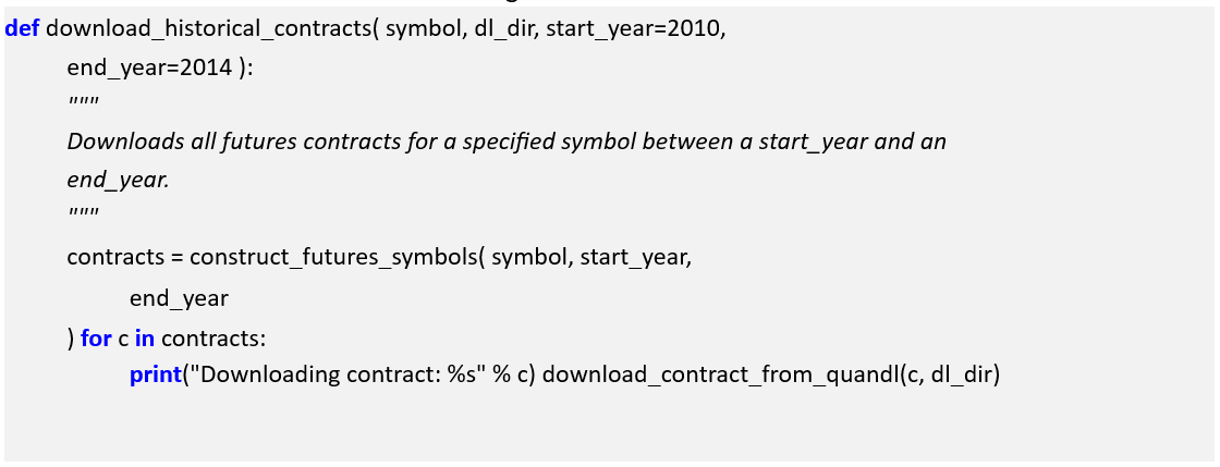
Now we tie the above two functions together to download all of the desired contracts:
Finally, we can add one of the futures prices to a pandas dataframe using the main function. We can then use matplotlib to plot the settle price:
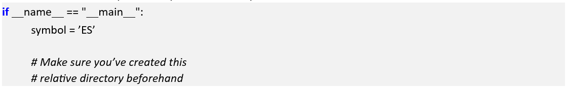
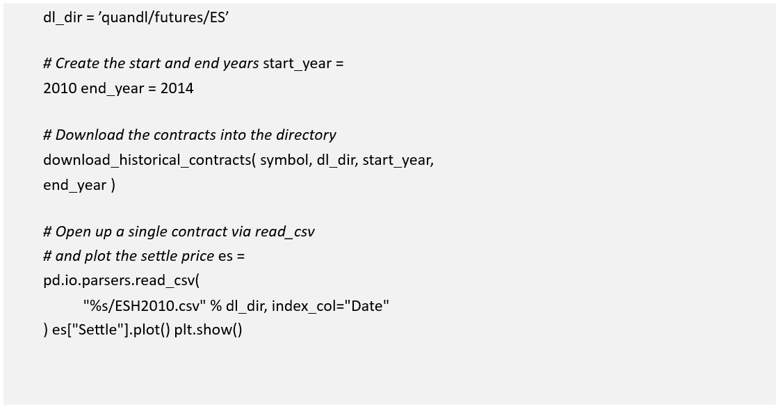
The output of the plot is given in Figure 2.
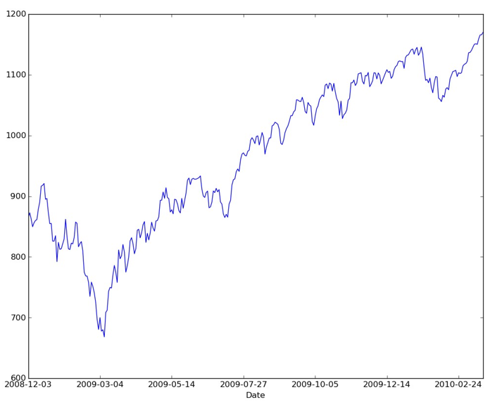
Figure 9: ESH2010 Settle Price
The above code can be modified to collect any combination of futures contracts from Quandl as necessary. Remember that unless a higher API request is made, the code will be limited to making 50 API requests per day.
4.3] DTN IQFeed:
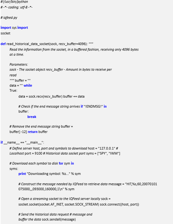
For those of you who possess a DTN IQFeed subscription, the service provides a client-server mechanism for obtaining intraday data. For this to work it is necessary to download the IQLink server and run it on Windows. Unfortunately, it is tricky to execute this server on Mac or Linux unless making use of the WINE emulator. However once the server is running it can be connected to via a socket at which point it can be queried for data.
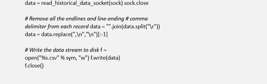
In this section we will obtain minutely bar data for a pair of US ETFs from January 1st 2007 onwards using a Python socket interface. Since there are approximately 252 trading days within each year for US markets, and each trading day has 6.5 hours of trading, this will equate to at least 650,000 bars of data, each with seven data points: Timestamp, Open, Low, High, Close, Volume and Open Interest.
I have chosen the SPY and IWM ETFs to download to CSV. Make such to start the IQLink program in Windows before executing this script:
With additional subscription options in the DTN IQFeed account, it is possible to download individual futures contracts (and back-adjusted continuous contracts), options and indices. DTN IQFeed also provides real-time tick streaming, but this form of data falls outside the scope.
5.) Cleaning Financial Data
Subsequent to the delivery of financial data from vendors it is necessary to perform data cleansing. Unfortunately this can be a painstaking process, but a hugely necessary one. There are multiple issues that require resolution: Incorrect data, consideration of data aggregation and backfilling. Equities and futures contracts possess their own unique challenges that must be dealt with prior to strategy research, including back/forward adjustment, continuous contract stitching and corporate action handling.
5.1] Data Quality:
The reputation of a data vendor will often rest on its (perceived) data quality. In simple terms, bad or missing data leads to erroneous trading signals and thus potential loss. Despite this fact, many vendors are still plagued with poor or inconsistent data quality. Thus there is always a cleansing process necessary to be carried.
The main culprits in poor data quality are conflicting/incorrect data, opaque aggregation of multiple data sources and error correction (“backfilling”).
Conflicting and Incorrect Data
Bad data can happen anywhere in the stream. Bugs in the software at an exchange can lead to erroneous prices when matching trades. This filters through to the vendor and subsequently the trader. Reputable vendors will attempt to flag upstream “bad ticks” and will often leave the “correction” of these points to the trader.
5.2] Continuous Futures Contracts:
In this section we are going to discuss the characteristics of futures contracts that present a data challenge from a backtesting point of view. In particular, the notion of the “continuous contract”. We will outline the main difficulties of futures and provide an implementation in Python with pandas that can partially alleviate the problems.
Brief Overview of Futures Contracts
Futures are a form of contract drawn up between two parties for the purchase or sale of a quantity of an underlying asset at a specified date in the future. This date is known as the delivery or expiration. When this date is reached the buyer must deliver the physical underlying (or cash equivalent) to the seller for the price agreed at the contract formation date.
In practice futures are traded on exchanges (as opposed to Over The Counter – OTC trading) for standardised quantities and qualities of the underlying. The prices are marked to market every day. Futures are incredibly liquid and are used heavily for speculative purposes. While futures were often utilised to hedge the prices of agricultural or industrial goods, a futures contract can be formed on any tangible or intangible underlying such as stock indices, interest rates of foreign exchange values.
A detailed list of all the symbol codes used for futures contracts across various exchanges can be found on the CSI Data site: Futures Factsheet.
The main difference between a futures contract and equity ownership is the fact that a futures contract has a limited window of availability by virtue of the expiration date. At any one instant there will be a variety of futures contracts on the same underlying all with varying dates of expiry. The contract with the nearest date of expiry is known as the near contract. The problem we face as quantitative traders is that at any point in time we have a choice of multiple contracts with which to trade. Thus we are dealing with an overlapping set of time series rather than a continuous stream as in the case of equities or foreign exchange.
The goal of this section is to outline various approaches to constructing a continuous stream of contracts from this set of multiple series and to highlight the tradeoffs associated with each technique.
Forming a Continuous Futures Contract
The main difficulty with trying to generate a continuous contract from the underlying contracts with varying deliveries is that the contracts do not often trade at the same prices. Thus situations arise where they do not provide a smooth splice from one to the next. This is due to contango and backwardation effects. There are various approaches to tackling this problem, which we now discuss.
Unfortunately there is no single “standard” method for joining futures contracts together in the financial industry. Ultimately the method chosen will depend heavily upon the strategy employing the contracts and the method of execution. Despite the fact that no single method exists there are some common approaches:
The Back/Forward (“Panama”) Adjustment method alleviates the “gap” across multiple contracts by shifting each contract such that the individual deliveries join in a smooth manner to the adjacent contracts. Thus the open/close across the prior contracts at expiry matches up.
The key problem with the Panama method includes the introduction of a trend bias, which will introduce a large drift to the prices. This can lead to negative data for sufficiently historical contracts. In addition there is a loss of the relative price differences due to an absolute shift in values. This means that returns are complicated to calculate (or just plain incorrect).
The Proportionality Adjustment approach is similar to the adjustment methodology of handling stock splits in equities. Rather than taking an absolute shift in the successive contracts, the ratio of the older settle (close) price to the newer open price is used to proportionally adjust the prices of historical contracts. This allows a continous stream without an interruption of the calculation of percentage returns.
The main issue with proportional adjustment is that any trading strategies reliant on an absolute price level will also have to be similarly adjusted in order to execute the correct signal. This is a problematic and error-prone process. Thus this type of continuous stream is often only useful for summary statistical analysis, as opposed to direct backtesting research.
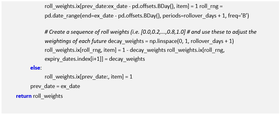
The Rollover/Perpetual Series method creates a continuous contract of successive contracts by taking a linearly weighted proportion of each contract over a number of days to ensure a smoother transition between each.
For example consider five smoothing days. The price on day 1, P1, is equal to 80% of the far contract price (F1) and 20% of the near contract price (N1). Similarly, on day 2 the price is
P2 = 0.6 × F2 + 0.4 × N2. By day 5 we have P5 = 0.0 × F5 + 1.0 × N5 = N5 and the contract then just becomes a continuation of the near price. Thus after five days the contract is smoothly transitioned from the far to the near.
The problem with the rollover method is that it requires trading on all five days, which can increase transaction costs. There are other less common approaches to the problem but we will avoid them here.
The remainder of the section will concentrate on implementing the perpetual series method as this is most appropriate for backtesting. It is a useful way to carry out strategy pipeline research.
We are going to stitch together the WTI Crude Oil “near” and “far” futures contract (symbol CL) in order to generate a continuous price series. At the time of writing (January 2014), the near contract is CLF2014 (January) and the far contract is CLG2014 (February).
In order to carry out the download of futures data I’ve made use of the Quandl plugin. Make sure to set the correct Python virtual environment on your system and install the Quandl package by typing the following into the terminal:
( pip install Quandl )
Now that the Quandl package is intalled, we need to make use of NumPy and pandas in order to carry out the rollover construction. Create a new file and enter the following import statements:
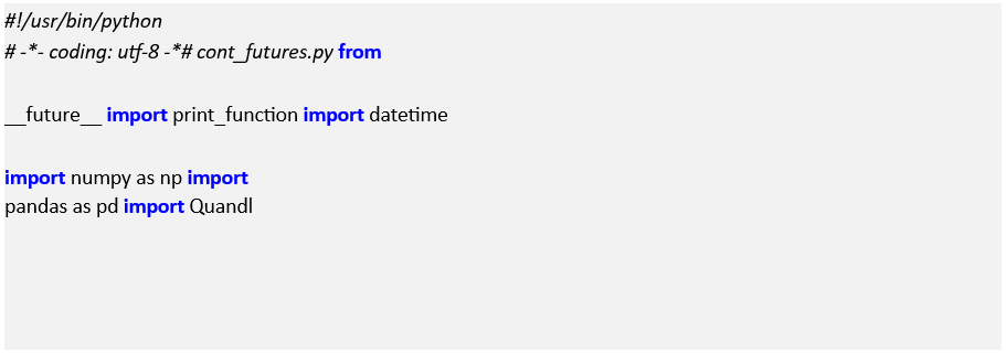
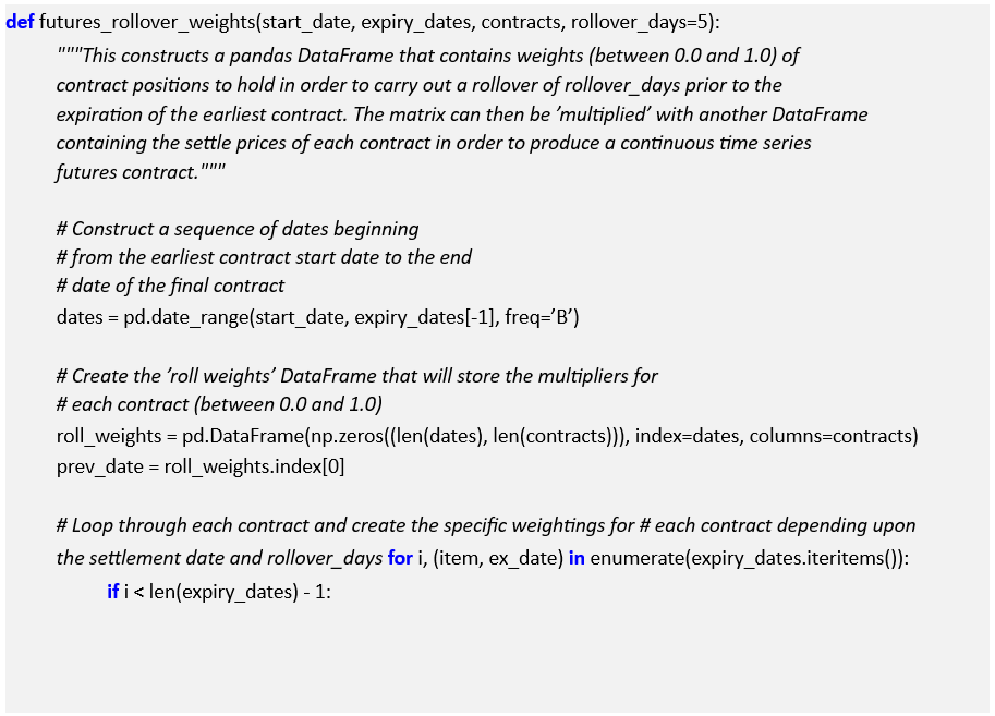
The main work is carried out in the futures_rollover_weights function. It requires a starting date (the first date of the near contract), a dictionary of contract settlement dates (expiry_dates), the symbols of the contracts and the number of days to roll the contract over (defaulting to five). The comments below explain the code:
Now that the weighting matrix has been produced, it is possible to apply this to the individual time series. The main function downloads the near and far contracts, creates a single DataFrame for both, constructs the rollover weighting matrix and then finally produces a continuous series of both prices, appropriately weighted:

The output is as follows:
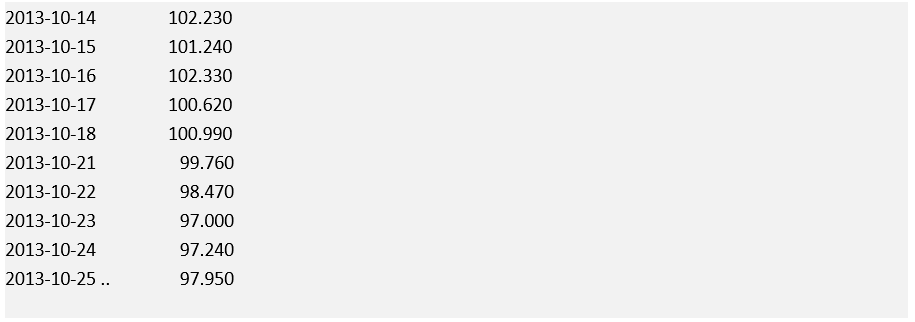
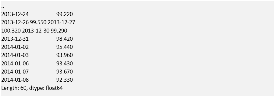
It can be seen that the series is now continuous across the two contracts. This can be extended to handle multiple deliveries across a variety of years, depending upon your backtesting needs.
Read Also; Financial Data Storage: Algorithmic Trading