Hurst Exponent and Variance Ratio Test
Intuitively speaking, a “stationary” price series means that the prices diff use from its initial value more slowly than a geometric random walk would. Mathematically, we can determine the nature of the price series by measuring this speed of diffusion. The speed of diffusion can be characterized by the variance;
Var(τ) = 〈|z(t + τ) − z(t)|2〉
where z is the log prices (z = log( y)), τ is an arbitrary time lag, and 〈…〉 is an average over all t’s. For a geometric random walk, we know that;
〈|z(t + τ) − z(t)|2〉 ∼ τ
The ∼ means that this relationship turns into an equality with some proportionality constant for large τ, but it may deviate from a straight line for small τ. But if the (log) price series is mean reverting or trending (i.e., has positive correlations between sequential price moves), Equation 2.3 won’t hold. Instead, we can write:
〈|z(t + τ) − z(t)|2〉 ∼ τ2H
where we have defined the Hurst exponent H. For a price series exhibiting geometric random walk, H = 0.5. But for a mean-reverting series, H < 0.5, and for a trending series, H > 0.5. As H decreases toward zero, the price series is more mean reverting, and as H increases toward 1, the price series is increasingly trending; thus, H serves also as an indicator for the degree of mean reversion or trendiness.
In Example, we computed the Hurst exponent for the same currency rate series USD.CAD that we used in the previous section using the MATLAB code. It generates an H of 0.49, which suggests that the price series is weakly mean reverting.
Example: Computing the Hurst Exponent
Using the same USD.CAD price series in the previous example, we now compute the Hurst exponent using a function called genhurst we can download from MATLAB Central (www.mathworks.com/matlabcentral/fi leexchange/30076-generalized-hurst-exponent). This function computes a generalized version of the Hurst exponent defined by 〈|z(t + τ) − z(t)|2q〉 ∼ τ2H(q), where q is an arbitrary number. But here we are only interested in q = 2, which we specify as the second input parameter to genhurst.
H=genhurst(log(y), 2);
If we apply this function to USD.CAD, we get H = 0.49, indicating that it may be weakly mean reverting.
Because of fi nite sample size, we need to know the statistical significance and MacKinlay of an estimated value of H to be sure whether we can reject the null hypothesis that H is really 0.5. This hypothesis test is provided by the Variance Ratio test.
The Variance Ratio Test simply tests whether;
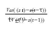
Is equal to 1. There is another ready-made MATLAB Econometrics Toolbox function v ratio test for this, whose usage I demonstrate in Example.
Example: Using the Variance Ratio Test for Stationarity
The vratiotest from MATALB Econometric Toolbox is applied to the same USD.CAD price series y that have been used in the previous examples in this chapter. The outputs are h and p Value: h = 1 means rejection of the random walk hypothesis at the 90 percent confidence level, h = 0 means it may be a random walk. p Value gives the probability that the null (random walk) hypothesis is true.
[h,pValue]=vratiotest(log(y));
We find that h = 0 and p Value = 0.367281 for USD.CAD, indicating that there is a 37 percent chance that it is a random walk, so we cannot reject this hypothesis.
Read Also; How the Augmented Dickey-Fuller Test Enhances Algorithmic Trading Strategies