
Augmented Dickey-Fuller Test
If a price series is mean reverting, then the current price level will tell us something about what the price’s next move will be: If the price level is higher than the mean, the next move will be a downward move; if the price level is lower than the mean, the next move will be an upward move. The ADF test is based on just this observation.
We can describe the price changes using a linear model:
Δy(t) = λy(t − 1) + μ + βt + α1Δy(t − 1) + … + αkΔy(t − k) + t
where Δy(t) ≡ y(t) − y(t − 1), Δy(t − 1) ≡ y(t − 1) − y(t − 2), and so on. The ADF test will find out if λ = 0. If the hypothesis λ = 0 can be rejected, that means the next move Δy(t) depends on the current level y(t − 1), and therefore it is not a random walk. The test statistic is the regression coefficient λ (with y(t − 1) as the independent variable and Δy(t) as the dependent variable) divided by the standard error of the regression fi t: λ/SE(λ). The statisticians Dickey and Fuller have kindly found out for us the distribution of this test statistic and tabulated the critical values for us, so we can look up for any value of λ/SE(λ) whether the hypothesis can be rejected at, say, the 95 percent probability level.
Notice that since we expect mean regression, λ/SE(λ) has to be negative, and it has to be more negative than the critical value for the hypothesis to be rejected. The critical values themselves depend on the sample size and whether we assume that the price series has a non-zero mean −μ/λ or a steady drift −βt/λ. In practical trading, the constant drift in price, if any, tends to be of a much smaller magnitude than the daily fluctuations in price. So for simplicity we will assume this drift term to be zero (β = 0).
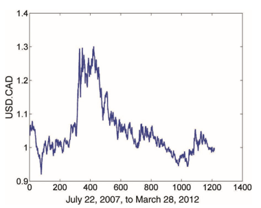
In Example, we apply the ADF test to a currency rate series USD.CAD.
1. Example:
The ADF function has three inputs. The first is the price series in ascending order of time (chronological order is important). The second is a parameter indicating whether we should assume the off set μ and whether the drift β in Equation 2.1 should be zero. We should assume the off set is nonzero, since the mean price toward which the prices revert is seldom zero. We should, however, assume the drift is zero, because the constant drift in price tends to be of a much smaller magnitude than the daily fluctuations in price. These considerations mean that the second parameter should be 0 (by the package designer’s convention). The third input is the lag k. You can start by trying k = 0, but often only by setting k = 1 can we reject the null hypothesis, meaning that the change in prices often does have serial correlations. We will try the test on the exchange rate USD.CAD (how many Canadian dollars in exchange for one U.S. dollar). We assume that the daily prices at 17:00 ET are stored in a MATLAB array γ. The data fi le is that of one-minute bars, but we will just extract the end-of-day prices at 17:00 ET. Sampling the data at intraday frequency will not increase the statistical significance of the ADF test. We can see from Figure 2.2 that it does not look very stationary.
2. Example:
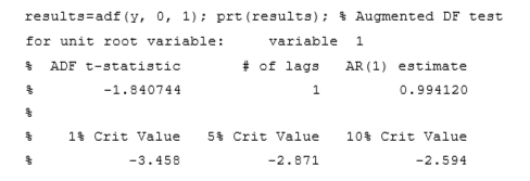
And indeed, you should find that the ADF test statistic is about −1.84, but the critical value at the 90 percent level is −2.594, so we can’t reject the hypothesis that λ is zero. In other words, we can’t show that USDCAD is stationary, which perhaps is not surprising, given that the Canadian dollar is known as a commodity currency, while the U.S. dollar is not. But note that λ is negative, which indicates the price series is at least not trending.
Read Also; Mean Reversion Explained: A Beginner’s Guide to This Powerful Trading Strategy