Algorithmic Trading Strategies In Cryptocurrency

1.) Moving Average

The moving average is the building block of all the strategies discussed in this paper. While a moving average does not entail a trading strategy on its own, it forms an integral part of all the other trading strategies. A moving average has a numeric value associated with it. If the numeric value is represented as x, the moving average vould be called the x-day moving average. Some common examples are a 5-day moving average, 10-day moving average, or 20-day moving. average

An x-day moving average is calculated by adding together the prices of the security for the last x days and dividing that total value by x. This finds the average price over the last x days. For example, a 5-day moving average would be calculated by adding the price of the security over the last five days and dividing the sum total by 5. The formula for calculating a moving average is as follows:

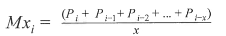
In the equation, represents the current day, i-1 represents the day before the current day, end i-x represents x days before the current day. Mx, represents the x-day moving average at i, the current point in time. / represents the price on the current day. represents the price on the day before the current day. P represents the price two days before the current day, and P., represents the price x days before the current day.

For use in this paper, the abbreviation “mva” will refer to moving average.

2.) Taking Moving Average to Minutes

The standard moving averages used for the stock market are the 50-day. 100-day, and 200-day moving averages. However, when this was tried with cryptocurrency, the results were poor. Because of cryptocurrency’s volatile nature, the moving average was far too large and did not trigger any buy or sell signals for the algorithm. Therefore, the moving average periods have to be much shorter. All of the algorithms detailed in this paper use a moving average increment of less than ten days. Normally, an x-day moving average would only take in x data points to calculate each moving average, as seen in the formula above. However, using merely ten data points is not likely to produce a very accurate result. This is because the fewer the data points in the moving average, the more sharply the average will change. This will result in the algorithm being less accurate, leading to poor trading results.

To keep the moving average accurate and responsive to price changes without using a longer time increment, moving average values were taken in increments of minutes, rather than days. Several values were tried for moving average increments in minutes, but the one used for a majority of the research was 5-minute increments.

Using 5-minute increments means that a 1-day moving average will actually be a 288-increment moving average, where each increment is five minutes. Therefore, to calculate a 1-day moving average, the last 288 price points will be taken over increments of five minutes, and those will all be added and divided by 288. This paper still refers to the strategies in terms of day increments, such as a 1-day moving average, instead of a 288 times 5-minute moving average. However, when reading this paper, it is important to remember that every moving average is actually done in increments of five minutes.

3.) Simple Moving Average Crossover

The first strategy used in this research is the Simple Moving Average Crossover. This trategy is also the simplest strategy used in this paper, as it only uses the moving average and the current price.

The Simple Moving Average Crossover Strategy calculates the x-day moving average and compares it to the current price. Whenever the current price crosses the the x’day moving average, the algorithm will trigger a buy or sell signal. Crossing the x-day moving average is defined as moving from below the moving average to above the moving average, or vice versa. Since the moving average changes very slowly when compared to the current price, it is always said that the price crosses the moving average, instead of the moving average crossing the price.

The price crossing above the moving average is defined as an instance in time where the price is greater than the moving average and the price was less than the moving average in the last instance of time. Since the increments of time used in this research are five minutes, the price crossing above the moving average refers to when the price is greater than the moving average but was less than the moving average five minutes before.

Conversely, the price crossing below the moving average is defined as an instance in time when the price is less than the moving average and the price was greater than the moving average five minutes before.

When the price crosses above the moving average, the Simple Moving Average Crossover algorithm will trigger a buy signal and the security will be bought. When the price crosses above the moving average, this predicts that the price of the security will continue to increase. This is because the moving average reacts slowly to the price’s change, so any immediate change in price has the potential to bring the price above or below the moving average’s value. Ideally, the moving average would be positioned properly so that most small changes in value. do not cross the moving average’s value and are filtered out by the algorithm. In this case, only big enough changes in the price’s value will cross the moving average’s line, triggering a buy or sell signal.

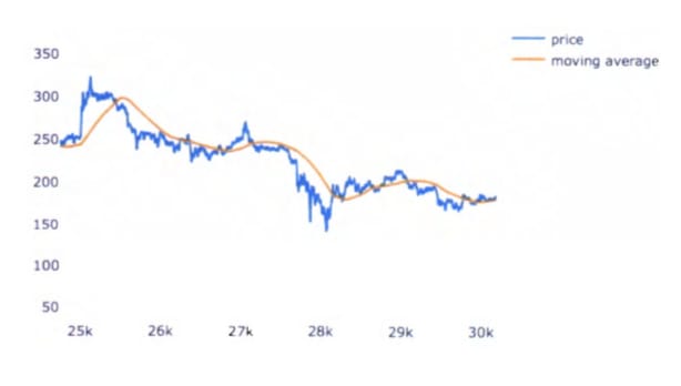
Figure.1 Litecoin’s price with a 1.7-day moving average.

Figure 1, shown on the previous page, plots the price against the moving average. The blue line represents the current price at each point in time, and the orange line represents the moving average value at each point in time. The y-axis represents the current price in United States Dollars, and the x-axis represents time. Each unit of time is a 5-minute interval, starting at 6:40pm on October 5, 2017. On the graph above, the x-axis values range from 25k to 30k. The value of 25k on the graph represents 25,000 5-minute intervals after 6:40pm on October 5, 2017, or 125,000 minutes after 6:40pm on October 5. Since there are 1,440 minutes each day, 125,000 minutes is approximately 89 days. Eighty-nine days after October 5, 2017, is January 2, 2018. The value of 30,000 on the right side of the graph represents 5,000 5-minute intervals, or 25,000 minutes after January 2, 2018. This is approximately 17 days, putting the 30k label on the x-axis around January 19, 2018.

The analogy of the price “crossing over” or “crossing under” the moving average can be seen here at any point where the two lines cross. It can be seen in the graph that the blue line changes much more than the orange line. That is because the actual price fluctuates greatly, while the moving average reacts much more slowly.

In Figure 1, the price crosses the moving average around an x-value of 27k. Since the price was greater than the moving average and then crossed below the moving average, this is a prediction that the price is heading down. The Simple Moving Average Crossover Strategy would sell Litecoin at that point in time in this scenario. When the two lines cross again, around the 28k mark on the x-axis, the price was above the moving average line and is crossing below the moving average line.

Since the algorithm would have sold around the 27k time and bought again around the 28k time, the user of the algorithm would not have had any holdings in Litecoin during that time and would have held only USD. This would have avoided much of Litecoin’s drop in price during that time, since the algorithm would not own any Litecoin at the time of the drop in price.

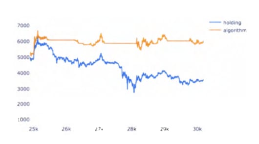
Figure 2. Algorithm (1.7-day mva) vs. holding Litecoin.

Figure 2, shown above, displays graph of the amount of money that a person would have in two scenarios: the orange line represents the amount of money one would have when using the algorithm and the blue line represents the amount of money one would have merely holding Litecoin. Both scenarios assume that the person had invested $1000 on October 5, 2017. The x-axis has the same values as from Figure 1, from January 2 to January 19, 2018. Since the graph starts at 125,000 minutes after the initial $1000 was invested, both lines start on this graph much above that starting amount.

As can be seen in Figure 2, the line representing the algorithm’s value is completely horizontal between the 27k mark and the 28k mark. This is because the algorithm has all of its value in USD at that moment and nothing in Litecoin. Therefore, any changes in Litecoin’s price do not affect the algorithm and the value held by the algorithm remains constant. This is the goal of the Simple Moving Average Crossover Strategy: to hold only cryptocurrency and no USD when the price of the cryptocurrency is going up, and to hold only USD and no cryptocurrency when the price of the cryptocurrency is going down.

Figures 1 and 2 show that this trading strategy can work well enough to enable the algorithm to outperform merely buying and holding a cryptocurrency. However, the algorithm is not perfect because it sells Litecoin after the price starts to decline and buys Litecoin again after the price has started to increase. Ideally, the algorithm would sell right as the price starts to decline and buy right as the price starts to increase. While no algorithm is perfect, the goal of this research has been to find an algorithm that will come as close as possible to selling right before a dip in price and buying right before a rise in price. The following strategies all are improvements on the Simple Moving Average Crossover that attempt to come closer to the ideal algorithm of perfect buying and selling.

4.) Exponential Moving Average Crossover

As the name implies, the Exponential Moving Average Crossover Strategy is similar to the Simple Moving Average Crossover Strategy. The Exponential Moving Average Crossover Strategy is an improvement on the Simple Moving Average Crossover Strategy; it takes the same concept with respect to buying and selling when the price and moving average cross, but has a different formula to calculate the moving average at each increment of time.

A simple moving average is the moving average discussed in the “Moving Average” section above. The name is fitting, because it simply adds up the prices for a set number of days and then divides by the number of days. An exponential moving average improves on this strategy by putting more emphasis on more-recent days. The simple strategy does not take into consideration how long it has been since the price was current, as long as the price is not beyond the window of what it adds. The exponential strategy, however, puts more weight on more-recent prices and less weight on older prices.

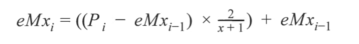
In the equation, represents the current point in time. 1-1 represents one time period (in this case, five minutes) before the current point in time, eMx, represents the x-period exponential moving average at the current point in time. Mx represents the exponential moving average five minutes before the current point in time. P, represents the price at the current point in time. Finally, x represents the number of time periods taken into consideration for the moving average. Since there are 1,440 time periods each day, a 1-day moving average would have result in an x-value of 1,440 for this equation.

This is a recursive equation, meaning that each iteration of the equation builds on the previous iteration. Purely using this equation doesn’t allow for the very first value to be calculated. The very first value is eMxs, since there have not been enough data points on every time instance before time instance to determine a moving average. For the very first value, eMx, a simple moving average will be used. For every instance of time after the first value, the exponential moving average formula will be used to calculate it.

To show how an exponential moving average weights the values toward more recent instances in time, a 5-interval moving average will be used. In a simple moving average, the prices of the last five time intervals are added up and the sum is divided by 5. Therefore, each price has a 20% influence on the moving average. With an exponential moving average the multiplier on the most recent price is, where is the number of intervals used in this exponential moving average. In this example, the number of intervals is 5, so the multiplier ist. thus the latest price has a 33% multiplier. Because of how the recursive formula is set up, the weighting on each value slowly diminishes as the values become less recent.

5.) Mean Reversion

The Mean Reversion Strategy is another improvement on the Simple Moving Average Crossover Strategy, but with a very different approach from the Exponential Moving Average Crossover Strategy. The exponential moving average attempted to improve the simple moving average by making a better moving average that would follow the changes in price more closely. The Mean Reversion Strategy still uses the simple moving average, but it attempts to predict the price’s decline before the price’s value crosses below the moving average’s value. It also attempts to predict the price’s rise before the price’s value crosses above the moving average’s value.

The Mean Reversion Strategy accomplishes this testing the price against two other values, instead of testing against the moving average. These two values are known as the upper bound and lower bound. The upper bound is placed a certain amount above the moving average line and the lower bound is placed a certain amount below the moving average line.

In addition to the moving average value, the Mean Reversion Strategy has another value called the offset. The offset is the amount that the bounds are offset from the moving average. For example, if the offset is x, then the upper bound will be at (100+ x)% of the moving average, and the lower bound will be at (100x)% of the moving average. Figure 3 demonstrates this below.

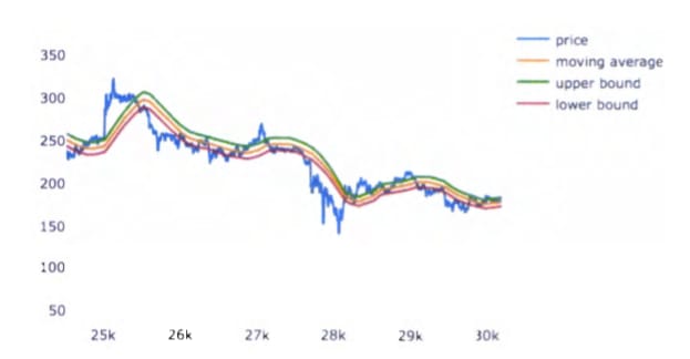
Figure 3. Mean Reversion on Litecoin’s price with a 1.7-day mva.

In Figure 3, shown above, the blue line represents Litecoin’s price. The orange line represents the 1.7-day moving average using 5-minute time intervals. The green line represents the upper bound with a 3% offset (103% of the moving average). The red line represents the lower bound at 97% of the moving average.

As can be seen on the graph, the price will cross the upper bound sooner after the price starts to decline than the moving average crossed. The same is also true with the lower bound: using the lower bound will detect a rise in price sooner than only using the moving average.

Mean Reversion is commonly used when a security’s price has fluctuations but returns to a similar price between fluctuations. This is where the name is from: the fact that the price of the security reverts to the mean. While cryptocurrency prices are extremely volatile and not the stable price that mean reversion would expect, this research attempted to determine if doing mean reversion on a small enough scale could be profitable. The reasoning behind this idea is that, even though the price is volatile, it is relatively stable in small enough time periods.

6.) Pairs Trading

All of the strategies discussed so far trade only one cryptocurrency back and forth with USD. At any point in time, the algorithm either has all of its value held in the cryptocurrency, or all of its value held in USD. These strategies attempt to gain value by holding the cryptocurrency when its price is increasing and they attempt to avoid losses by holding USD when the cryptocurrency’s price is decreasing. However, they make no attempt to gain value when the cryptocurrency’s price is falling.

This is where the Pairs Trading Strategy attempts to be different: it tries to find two cryptocurrencies that follow opposite trends. This way, if one cryptocurrency is rising while the other is falling and vice versa, the strategy can be gaining value almost all the time. The idea of the strategy is to perform a Mean Reversion Strategy, but instead of doing a mean reversion on the price, a mean reversion on the difference in prices is performed. At the beginning of the algorithm, the cryptocurrencies with the higher and lower prices are determined. Then, every time the mean reversion is calculated, the price is substituted with the difference between the higher and lower prices.

Mean reversion is used because the idea is that the difference in price will fluctuate but eventually return to the mean. The term cointegration refers to a situation when one of the securities’ prices has an effect on the other. This means that a rise in one price will cause a fall in the other price, or vice versa. If the two securities’ prices are truly cointegrated, this pairs trading strategy will work well.

Several tests can be used to determine how cointegrated two prices are. Three of the tests for cointegration include the Dickey-Fuller Test, the Augmented Dickey-Fuller Test, and the Johansen Cointegration Test. These are very important when finding usable pairs in the stock market, since the number of possible pairs is so large. It would require too much time to run the actual algorithm with every possible pair, so a test is needed to find good pairs.

However, when using only the top five cryptocurrencies, there are only 5C2 = 10 possible pairs. Therefore, there was no need to test each pair for cointegration when the actual algorithm could be tested on each pair easily. Each pair was tested and the effectiveness of the algorithm on each pair was used to determine the cointegration of the pair.