
Improve Your Backtesting Accuracy with Statistical Significance and Hypothesis Testing
The issue of finite sample size arises in any backtest since unpredictability affects all statistical measures we calculate, including maximum drawdowns and average returns. To put it another way, we might be fortunate that our approach was successful in a tiny sample of data. To deal with this problem, statisticians have created a general process known as hypothesis testing.
The general framework of hypothesis testing as applied to backtesting follows these steps:
- Based on a backtest on some finite sample of data, we compute a certain statistical measure called the test statistic. For concreteness, let’s say the test statistic is the average daily return of a trading strategy in that period.
- We suppose that the true average daily return based on an infinite data set is actually zero. This supposition is called the null hypothesis.
- We suppose that the probability distribution of daily returns is known. This probability distribution has a zero mean, based on the null hypothesis. We describe later how we determine this probability distribution.
- Based on this null hypothesis probability distribution, we compute the probability p that the average daily returns will be at least as large as the observed value in the backtest (or, for a general test statistic, as extreme, allowing for the possibility of a negative test statistic). This probability p is called the p-value, and if it is very small (let’s say smaller than 0.01), that means we can “reject the null hypothesis,” and conclude that the backtested average daily return is statistically significant.
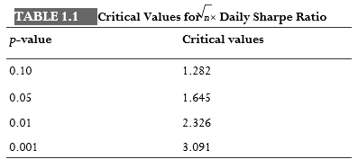
The step in this procedure that requires most thought is step 3. How do we determine the probability distribution under the null hypothesis? Perhaps we can suppose that the daily returns follow a standard parametric probability distribution such as the Gaussian distribution, with a mean of zero and a standard deviation given by the sample standard deviation of the daily returns. If we do this, it is clear that if the backtest has a high Sharpe ratio, it would be very easy for us to reject the null hypothesis. This is because the standard test statistic for a Gaussian distribution is none other than the average divided by the standard deviation and multiplied by the square root of the number of data points (Berntson, 2002). The p-values for various critical values are listed in Table 1.1. For example, if the daily Sharpe ratio multiplied by the square root of the number days ( n) in the backtest is greater than or equal to the critical value 2.326, then the p-value is smaller than or equal to 0.01.
This method of hypothesis testing is consistent with our belief that high Sharpe-ratio strategies are more statistically significant.
Another way to estimate the probability distribution of the null hypothesis is to use Monte Carlo methods to generate simulated historical price data and feed these simulated data into our strategy to determine the empirical probability distribution of profits. Our belief is that the profitability of the trading strategy captured some subtle patterns or correlations of the price series, and not just because of the first few moments of the price distributions. So if we generate many simulated price series with the same first moments and the same length as the actual price data, and run the trading strategy over all these simulated price series, we can find out in what fraction p of these price series are the average returns greater than or equal to the backtest return.
Ideally, p will be small, which allows us to reject the null hypothesis. Otherwise, the average return of the strategy may just be due to the market returns.
A third way to estimate the probability distribution of the null hypothesis is suggested by Andrew Lo and his collaborators (Lo, Mamaysky, and Wang, 2000). In this method, instead of generating simulated price data, we generate sets of simulated trades, with the constraint that the number of long and short entry trades is the same as in the backtest, and with the same average holding period for the trades. These trades are distributed randomly over the actual historical price series. We then measure what fraction of such sets of trades has average return greater than or equal to the backtest average return.
In Example 1.1, I compare these three ways of testing the statistical significance of a backtest on a strategy. We should not be surprised that they give us different answers, since the probability distribution is different in each case, and each assumed distribution compares our strategy against a different benchmark of randomness.
Example 1.1: Hypothesis Testing on a Futures Momentum Strategy
We apply the three versions of hypothesis testing, each with a different probability distribution for the null hypothesis, on the backtest results of the TU momentum strategy. That strategy buys (sells) the TU future if it has a positive (negative) 12-month return, and holds the position for 1 month. We pick this strategy not only because of its simplicity, but because it has a fixed holding period. So for version 3 of the hypothesis testing, we need to randomize only the starting days of the long and short trades, with no need to randomize the holding periods.
The first hypothesis test is very easy. We assume the probability distribution of the daily returns is Gaussian, with mean zero as befitting a null hypothesis, and with the standard deviation given by the standard deviation of the daily returns given by our backtest. So if ret is the Tx1 MATLAB© array containing the daily returns of the strategy, the test statistic is just;
mean(ret)/std(ret)*sqrt(length(ret))
which turns out to be 2.93 for our data set. Comparing this test statistic with the critical values in Table 1.1 tells us that we can reject the null hypothesis with better than 99 percent probability.
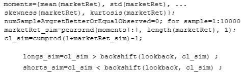
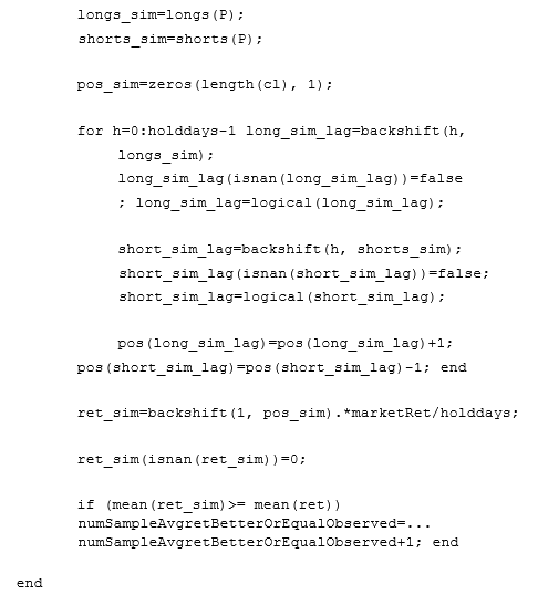
The second hypothesis test involves generating a set of random, simulated daily returns data for the TU future (not the daily returns of the strategy) for the same number of days as our backtest. These random daily returns data will have the same mean, standard deviation, skewness, and kurtosis as the observed futures returns, but, of course, they won’t have the same correlations embedded in them. If we find there is a good probability that the strategy can generate an as good as or better return on this random returns series as the observed returns series, it would mean that the momentum strategy is not really capturing any momentum or serial correlations in the returns at all and is profitable only because we were lucky that the observed returns’ probability distribution has a certain mean and a certain shape. To generate these simulated random returns with the prescribed moments, we use the pearsrnd function from the MATLAB Statistics Toolbox. After the simulated returns market Ret sim are generated, we then go on to construct a simulated price series cl sim using those returns. Finally, we run the strategy on these simulated prices and calculate the average return of the strategy. We repeat this 10,000 times and count how many times the strategy produces an average return greater than or equal to that produced on the observed data set.
Assuming that market Ret is the Tx1 array containing the observed daily returns of TU, the program fragment is displayed below.
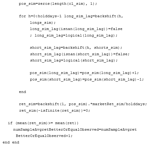
We found that out of 10,000 random returns sets, 1,166 have average strategy return greater than or equal to the observed average return. So the null hypothesis can be rejected with only 88 percent probability. Clearly, the shape of the returns distribution curve has something to do with the success of the strategy. (It is less likely that the success is due to the mean of the distribution since the position can be long or short at different times.)
The third hypothesis test involves randomizing the long and short entry dates, while keeping the same number of long trades and short trades as the ones in the backtest, respectively. We can accomplish this quite easily by the MATLAB function randperm:
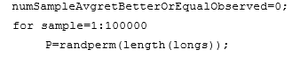
There is not a single sample out of 100,000 where the average strategy return is greater than or equal to the observed return. Clearly, the third test is much weaker for this strategy.
The fact that a null hypothesis is not unique and different null hypotheses can give rise to different estimates of statistical significance is one reason why many critics believe that hypothesis testing is a flawed methodology (Gill). The other reason is that we actually want to know the conditional probability that the null hypothesis is true given that we have observed the test statistic R: P(H0|R). But the procedure we outlined previously actually just computed the conditional probability of obtaining a test statistic R given that the null hypothesis is true: P(R|H0). Rarely is P(R|H0) = P(H0|R).
Even though hypothesis testing and the rejection of a null hypothesis may not be a very satisfactory way to estimate statistical significance, the failure to reject a null hypothesis can inspire very interesting insights. Our Example 1.1 shows that any random returns distribution with high kurtosis can be favorable to momentum strategies.
Read Also; Biggest Backtesting Mistakes in Algorithmic Trading and How to Avoid Them