Algo Trading Strategy Implementation

In this chapter we are going to consider the full implementation of trading strategies using the aforementioned event-driven backtesting system. In particular we will generate equity curves for all trading strategies using notional portfolio amounts, thus simulating the concepts of margin/leverage, which is a far more realistic approach compared to vectorised/returns based approaches.

The first set of strategies are able to be carried out with freely available data, either from Yahoo Finance, Google Finance or Quandl. These strategies are suitable for long-term algorithmic traders who may wish to only study the trade signal generation aspect of the strategy or even the full end-to-end system. Such strategies often possess smaller Sharpe ratios, but are far easier to implement and execute.

The latter strategy is carried out using intraday equities data. This data is often not freely available and a commercial data vendor is usually necessary to provide sufficient quality and quantity of data. I myself use DTN IQFeed for intraday bars. Such strategies often possess much larger Sharpe ratios, but require more sophisticated implementation as the high frequency requires extensive automation.

We will see that our first two attempts at creating a trading strategy on interday data are not altogether successful. It can be challenging to come up with a profitable trading strategy on interday data once transaction costs have been taken into account. The latter is something that many texts on algorithmic trading tend to leave out. However, it is my belief that as many factors as possible must be added to the backtest in order to minimises surprises going forward.

In addition, this book is primarily about how to effectively create a realistic interday or intraday backtesting system (as well as a live execution platform) and less about particular individual strategies. It is far harder to create a realistic robust backtester than it is to find trading strategies on the internet! While the first two strategies presented are not particularly attractive, the latter strategy (on intraday data) performs well and gives us confidence in using higher frequency data.

1.) Moving Average Crossover Strategy

I’m quite fond of the Moving Average Crossover technical system because it is the first nontrivial strategy that is extremely handy for testing a new backtesting implementation. On a daily timeframe, over a number of years, with long lookback periods, few signals are generated on a single stock and thus it is easy to manually verify that the system is behaving as would be expected.

In order to actually generate such a simulation based on the prior backtesting code we need to subclass the Strategy object as described in the previous chapter to create the MovingAverageCrossStrategy object, which will contain the logic of the simple moving averages and the generation of trading signals.

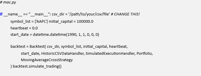
In addition we need to create the __main__ function that will load the Backtest object and actually encapsulate the execution of the program. The following file, mac.py, contains both of these objects.

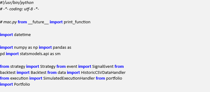
The first task, as always, is to correctly import the necessary components. We are importing nearly all of the objects that have been described in the previous chapter:

Now we turn to the creation of the MovingAverageCrossStrategy. The strategy requires both the bars DataHandler, the events Event Queue and the lookback periods for the simple moving averages that are going to be employed within the strategy. I’ve chosen 100 and 400 as the “short” and “long” lookback periods for this strategy.

The final attribute, bought, is used to tell the Strategy when the backtest is actually “in the market”. Entry signals are only generated if this is “OUT” and exit signals are only ever generated if this is “LONG” or “SHORT”:

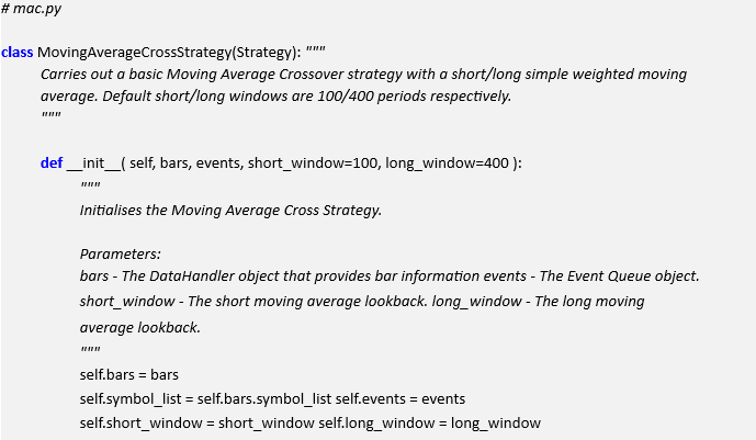
# Set to True if a symbol is in the market self.bought = self._calculate_initial_bought()

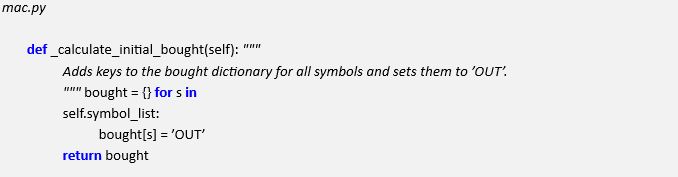
Since the strategy begins out of the market we set the initial “bought” value to be “OUT”, for each symbol:

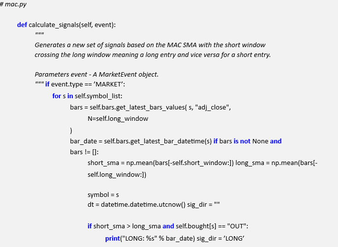
The core of the strategy is the calculate^_signals method. It reacts to a MarketEvent object and for each symbol traded obtains the latest N bar closing prices, where N is equal to the largest lookback period.

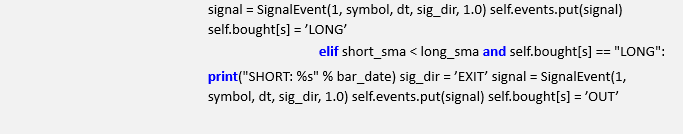
It then calculates both the short and long period simple moving averages. The rule of the strategy is to enter the market (go long a stock) when the short moving average value exceeds the long moving average value. Conversely, if the long moving average value exceeds the short moving average value the strategy is told to exit the market.

This logic is handled by placing a SignalEvent object on the events Event Queue in each of the respective situations and then updating the “bought” attribute (per symbol) to be “LONG” or “OUT”, respectively. Since this is a long-only strategy, we won’t be considering “SHORT” positions:

That concludes the MovingAverageCrossStrategy object implementation. The final task of the entire backtesting system is populate a main method in mac.py to actually execute the backtest.

Firstly, make sure to change the value of csv_dir to the absolute path of your CSV file directory for the financial data. You will also need to download the CSV file of the AAPL stock (from Yahoo Finance), which is given by the following link (for Jan 1st 1990 to Jan 1st 2002), since this is the stock we will be testing the strategy on: http://ichart.finance.yahoo.com/table.csv?s=AAPL&a=00&b=1&c=1990&d=00&e=1 &f=2002&g=d&ignore=.csv

Make sure to place this file in the path pointed to from the main function in csv_dir.

The main function simply instantiates a new backtest object and then calls the simulate_trading method on it to execute it:

To run the code, make sure you have already set up a Python environment (as described in the previous chapters) and then navigate the directory where your code is stored. You should simply be able to run:

python mac.py

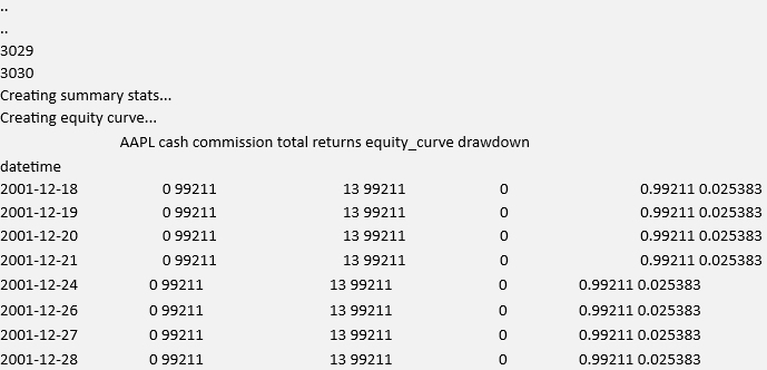
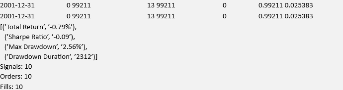
You will see the following listing (truncated due to the bar count printout!):

The performance of this strategy can be seen in Fig.1:

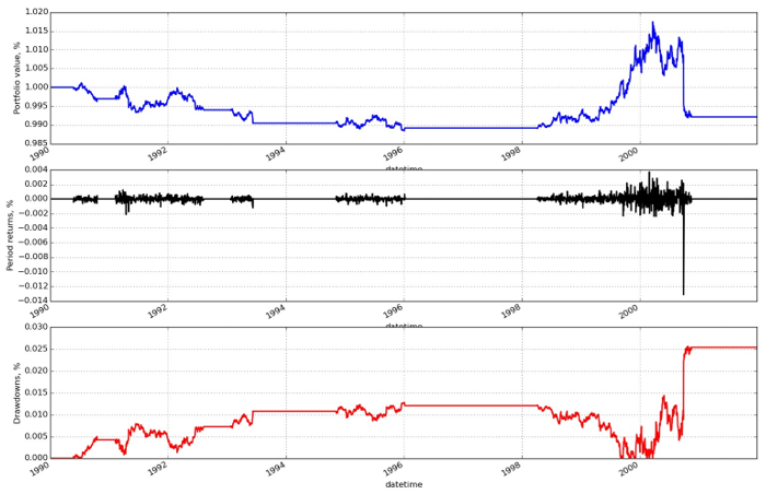
Figure .1: Equity Curve, Daily Returns and Drawdowns for the Moving Average Crossover strategy

Evidently the returns and Sharpe Ratio are not stellar for AAPL stock on this particular set of technical indicators! Clearly we have some work to do in the next set of strategies to find a system that can generate positive performance.

2.) S&P500 Forecasting Trade

In this sectiuon we will consider a trading strategy built around the forecasting engine discussed in prior chapters. We will attempt to trade off the predictions made by a stock market forecaster.

We are going to attempt to forecast SPY, which is the ETF that tracks the value of the S&P500. Ultimately we want to answer the question as to whether a basic forecasting algorithm using lagged price data, with slight predictive performance, provides us with any benefit over a buy-and-hold strategy.

The rules for this strategy are as follows:

Fit a forecasting model to a subset of S&P500 data. This could be Logistic Regression, a Discriminant Analyser (Linear or Quadratic), a Support Vector Machine or a Random Forest. The procedure to do this was outlined in the Forecasting chapter.
Use two prior lags of adjusted closing returns data as a predictor for tomorrow’s returns. If the returns are predicted as positive then go long. If the returns are predicted as negative then exit. We’re not going to consider short selling for this particular strategy.

Implementation

For this strategy we are going to create the snp_forecast.py file and import the following necessary libraries:

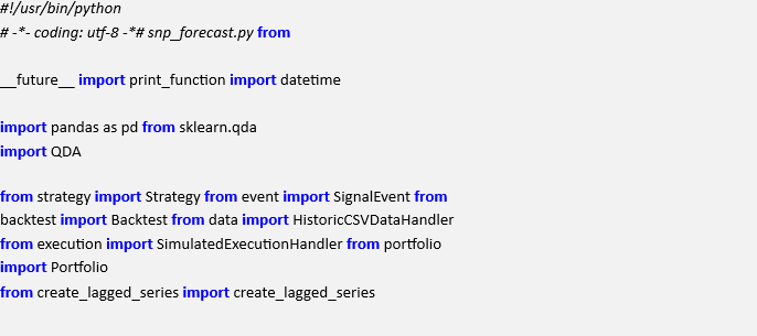
We have imported Pandas and Scikit-Learn in order to carry out the fitting procedure for the supervised classifier model. We have also imported the necessary classes from the event-driven backtester. Finally, we have imported the create^_lagged^_series function, which we used in the Forecasting chapter.

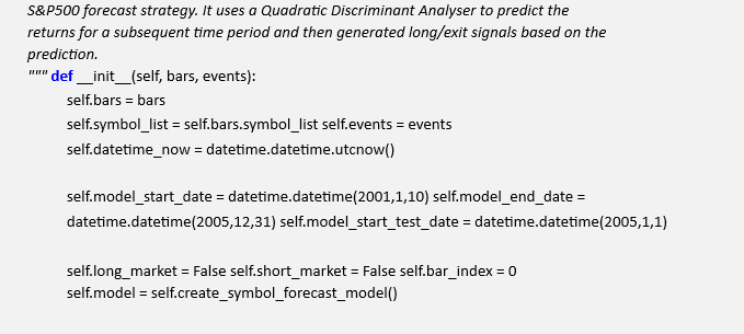
The next step is to create the SPYDailyForecastStrategy as a subclass of the Strategy abstract base class. Since we will “hardcode” the parameters of the strategy directly into the class, for simplicity, the only parameters necessary for the __init__ constructor are the bars data handler and the events queue.

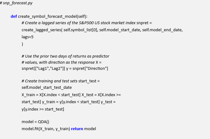
We set the self.model__***start/end/test dates as datetime objects and then tell the class that we are out of the market (self.long^_market = False). Finally, we set self.model to be the trained model from the create^_symbol^_forecast^_model below:

Here we define the create_symbol_forecast_model. It essentially calls the create_lagged_series function, which produces a Pandas DataFrame with five daily returns lags for each current predictor. We then consider only the two most recent of these lags. This is because we are making the modelling decision that the predictive power of earlier lags is likely to be minimal.

At this stage we create the training and test data, the latter of which can be used to test our model if we wish. I have opted to not output testing data, since we have already trained the model before in the Forecasting chapter. Finally we fit the training data to the Quadratic Discriminant Analyser and then return the model.

Note that we could easily replace the model with a Random Forest, Support Vector Machine or Logistic Regression, for instance. All we need to do is import the correct library from ScikitLearn and simply replace the model = QDA() line:

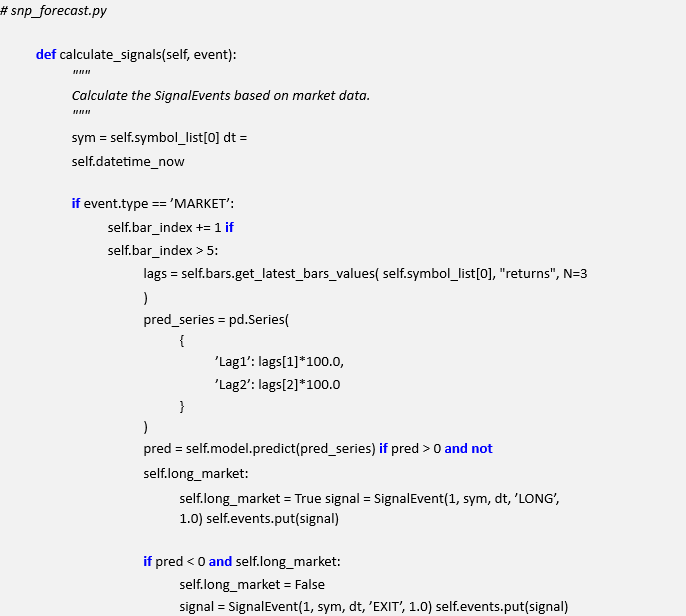
At this stage we are ready to override the calculate^_signals method of the Strategy base class. We firstly calculate some convenience parameters that enter our SignalEvent object and then only generate a set of signals if we have received a MarketEvent object (a basic sanity check).

We wait for five bars to have elapsed (i.e. five days in this strategy!) and then obtain the lagged returns values. We then wrap these values in a Pandas Series so that the predict method of the model will function correctly. We then calculate a prediction, which manifests itself as a +1 or -1.

If the prediction is a +1 and we are not already long the market, we create a SignalEvent to go long and let the class know we are now in the market. If the prediction is -1 and we are long the market, then we simply exit the market:

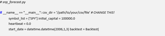
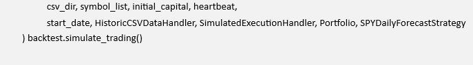
In order to run the strategy you will need to download a CSV file from Yahoo Finance for SPY and place it in a suitable directory (note that you will need to change your path below!). We then wrap the backtest up via the Backtest class and carry out the test by calling simulate^_trading:

The output of the strategy is as follows and is net of transaction costs:

The following visualisation in Fig 15.2 shows the Equity Curve, the Daily Returns and the Drawdown of the strategy as a function of time:

Note immediately that the performance is not great! We have a Sharpe Ratio < 1 but a reasonable drawdown of just under 6%. It turns out that if we had simply bought and held SPY in this time period we would have performed similarly, if slightly worse.

Hence we have not actually gained very much from our predictive strategy once transaction costs are included. I specifically wanted to include this example because it uses an “end to end” realistic implementation of such a strategy that takes into account conservative, realistic transaction costs. As can be seen it is not easy to make a predictive forecaster on daily data that produces good performance!

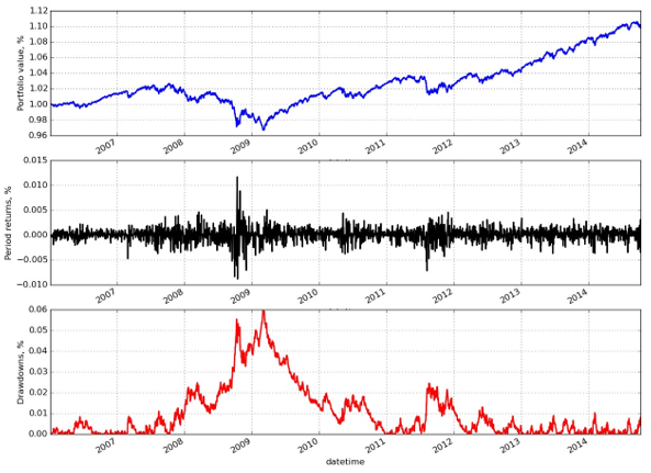
Figure .2: Equity Curve, Daily Returns and Drawdowns for the SPY forecast strategy

Our final strategy will make use of other time series and a higher frequency. We will see that performance can be improved dramatically after modifying certain aspects of the system.

3.) Mean-Reverting Equity Pairs Trade

In order to seek higher Sharpe ratios for our trading, we need to consider higher-frequency intraday strategies.

The first major issue is that obtaining data is significantly less straightforward because high quality intraday data is usually not free. As stated above I use DTN IQFeed for intraday minutely bars and thus you will need your own DTN account to obtain the data required for this strategy.

The second issue is that backtesting simulations take substantially longer, especially with the event-driven model that we have constructed here. Once we begin considering a backtest of a diversified portfolio of minutely data spanning years, and then performing any parameter optimisation, we rapidly realise that simulations can take hours or even days to calculate on a modern desktop PC. This will need to be factored in to your research process.

The third issue is that live execution will now need to be fully automated since we are edging into higher-frequency trading. This means that such execution environments and code must be highly reliable and bug-free, otherwise the potential for significant losses can occur.

This strategy expands on the previous interday strategy above to make use of intraday data.

In particular we are going to use minutely OHLCV bars, as opposed to daily OHLCV. The rules for the strategy are straightforward:

Identify a pair of equities that possess a residuals time series which has been statistically identified as mean-reverting. In this case, I have found two energy sector US equities with tickers AREX and WLL.
Create the residuals time series of the pair by performing a rolling linear regression, for a particular lookback window, via the ordinary least squares (OLS) algorithm. This lookback period is a parameter to be optimised.
Create a rolling z-score of the residuals time series of the same lookback period and use this to determine entry/exit thresholds for trading signals.
If the upper threshold is exceeded when not in the market then enter the market (long or short depending on direction of threshold excess). If the lower threshold is exceeded when in the market, exit the market. Once again, the upper and lower thresholds are parameters to be optimised.

Indeed we could have used the Cointegrated Augmented Dickey-Fuller (CADF) test to identify an even more accurate hedging parameter. This would make an interesting extension of the strategy.

Implementation

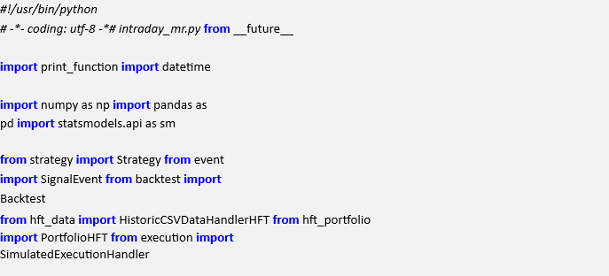
The first step, as always, is to import the necessary libraries. We require pandas for the rolling_apply method, which is used to apply the z-score calculation with a lookback window on a rolling basis. We import statsmodels because it provides a means of calculating the ordinary least squares (OLS) algorithm for the linear regression, necessary to obtain the hedging ratio for the construction of the residuals.

We also require a slightly modified DataHandler and Portfolio in order to carry out minutely bars trading on DTN IQFeed data. In order to create these files you can simply copy all of the code in portfolio.py and data.py into the new files hft^_portfolio.py and hft_data.py respectively and then modify the necessary sections, which I will outline below.

Here is the import listing for intraday^_mr.py:

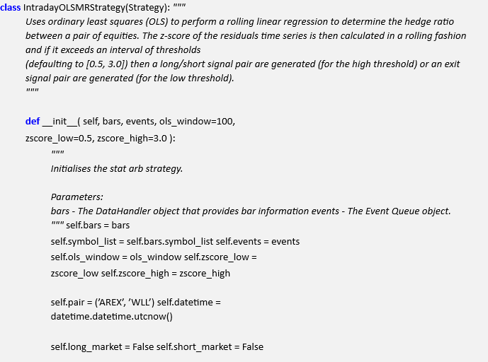
In the following snippet we create the IntradayOLSMRStrategy class derived from the Strategy abstract base class. The constructor ^__init^__method requires access to the bars historical data provider, the events queue, a zscore^_low threshold and a zscore^_high threshold, used to determine when the residual series between the two pairs is mean-reverting.

In addition, we specify the OLS lookback window (set to 100 here), which is a parameter that is subject to potential optimisation. At the start of the simulation we are neither long or short the market, so we set both self.long^_market and self.short^_market equal to False:

# intraday_mr.py

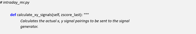
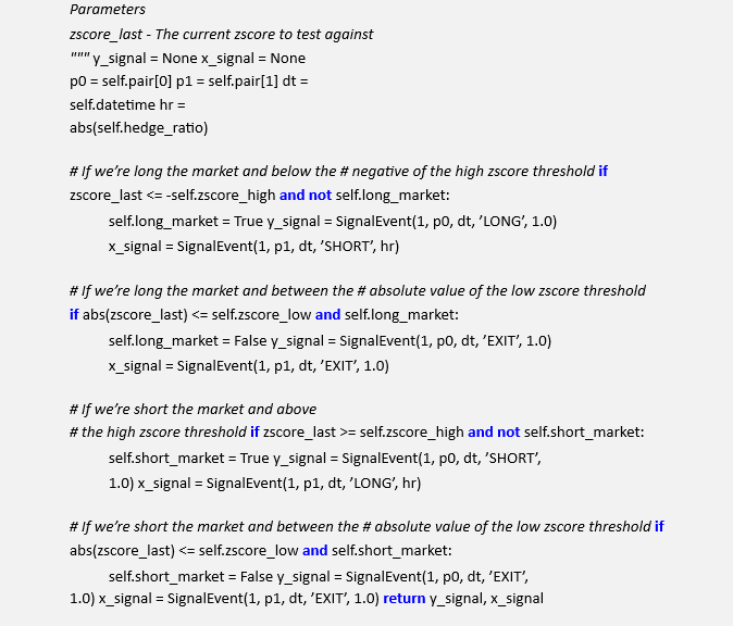
The following method, calculate^_xy^_signals, takes the current zscore (from the rolling calculation performed below) and determines whether new trading signals need to be generated.

These signals are then returned.

There are four potential states that we may be interested in. They are:

Long the market and below the negative zscore higher threshold
Long the market and between the absolute value of the zscore lower threshold
Short the market and above the positive zscore higher threshold
Short the market and between the absolute value of the zscore lower threshold

In either case it is necessary to generate two signals, one for the first component of the pair (AREX) and one for the second component of the pair (WLL). If none of these conditions are reached, then a pair of None values are returned:

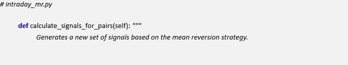
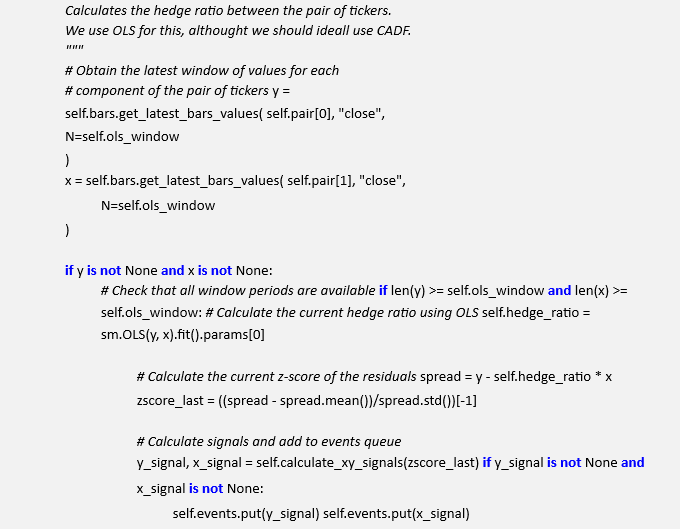
The following method, calculate^_signals^_for^_pairs obtains the latest set of bars for each component of the pair (in this case 100 bars) and uses them to construct an ordinary least squares based linear regression. This allows identification of the hedge ratio, necessary for the construction of the residuals time series.

Once the hedge ratio is constructed, a spread series of residuals is constructed. The next step is to calculate the latest zscore from the residual series by subtracting its mean and dividing by its standard deviation over the lookback period.

Finally, the y_signal and x_signal are calculated on the basis of this zscore. If the signals are not both None then the SignalEvent instances are sent back to the events queue:

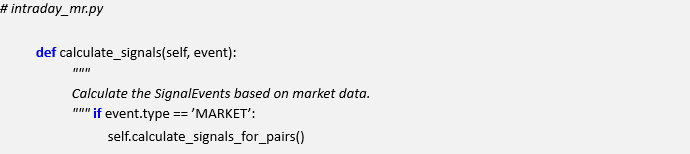
The final method, calculate_signals is overidden from the base class and is used to check whether a received event from the queue is actually a MarketEvent, in which case the calculation of the new signals is carried out:

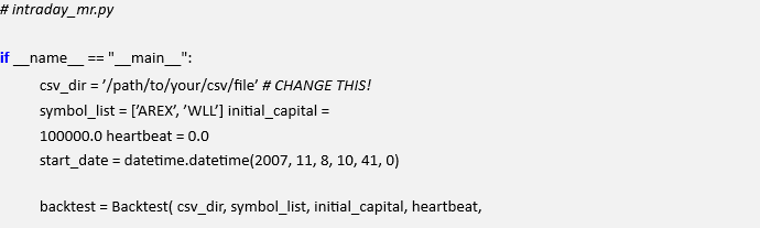
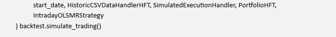
The __main__ section ties together the components to produce a backtest for the strategy. We tell the simulation where the ticker minutely data is stored. I’m using DTN IQFeed format. I truncated both files so that they began and ended on the same respective minute. For this particular pair of AREX and WLL, the common start date is 8th November 2007 at 10:41:00AM.

Finally, we build the backtest object and begin simulating the trading:

However, before we can execute this file we need to make some modifications to the data handler and portfolio objects.

In particular, it is necessary to create new files hft^_data.py and hft^_portfolio.py which are copies of data.py and portfolio.py respectively.

In hft_data.py we need to rename HistoricCSVDataHandler to HistoricCSVDataHandlerHFT and replace the names list in the ^_open^_convert^_csv^_files method. The old line is:

This must be replaced with:

This is to ensure that the new format for DTN IQFeed works with the backtester. The other change is to rename Portfolio to PortfolioHFT in hft_portfolio.py. We must then modify a few lines in order to account for the minutely frequency of the DTN data.

In particular, within the update_timeindex method, we must change the following code:

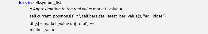
To:

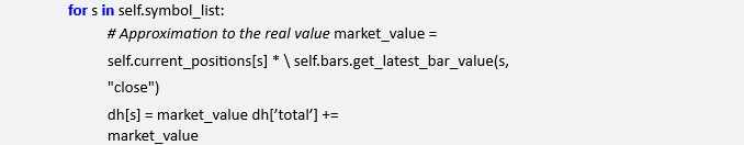
This ensures we obtain the close price, rather than the adj_close price. The latter is for Yahoo Finance, whereas the former is for DTN IQFeed.

We must also make a similar adjustment in update^_holdings^_from^_fill. We need to change the following code:

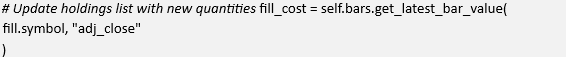
To:

The final change is occurs in the output^_summary^_stats method at the bottom of the file. We need to modify how the Sharpe Ratio is calculated to take into account minutely trading.

The following line:

sharpe_ratio = create_sharpe_ratio(returns)

Must be changed to:

sharpe_ratio = create_sharpe_ratio(returns, periods=252*6.5*60)

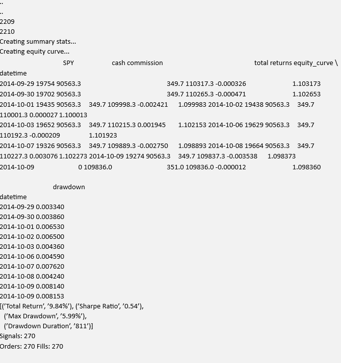
This completes the necessary changes. Upon execution of intraday_mr.py we get the following (truncated) output from the backtest simulation:

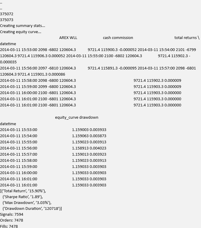
You can see that the strategy performs adequately well during this period. It has a total return of just under 16%. The Sharpe ratio is reasonable (when compared to a typical daily strategy), but given the high-frequency nature of the strategy we should be expecting more. The major attraction of this strategy is that the maximum drawdown is low (approximately 3%).

This suggests we could apply more leverage to gain more return.

The performance of this strategy can be seen in Fig 15.3:

Note that these figures are based on trading a total of 100 shares. You can adjust the leverage by simply adjusting the generate^_naive^_order method of the Portfolio class. Look for the mkt_quantity. It will be set to 100. Changing this to 2000, for instance, provides these results:

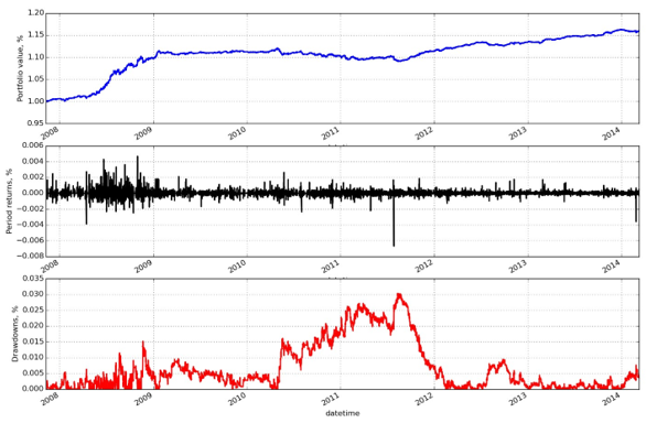
Figure .3: Equity Curve, Daily Returns and Drawdowns for intraday mean-reversion strategy attribute known as;

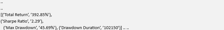
Clearly the Sharpe Ratio and Total Return are much more attractive, but we have to endure a 45% maximum drawdown over this period as well!

4.) Plotting Performance

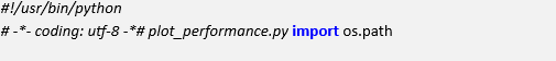
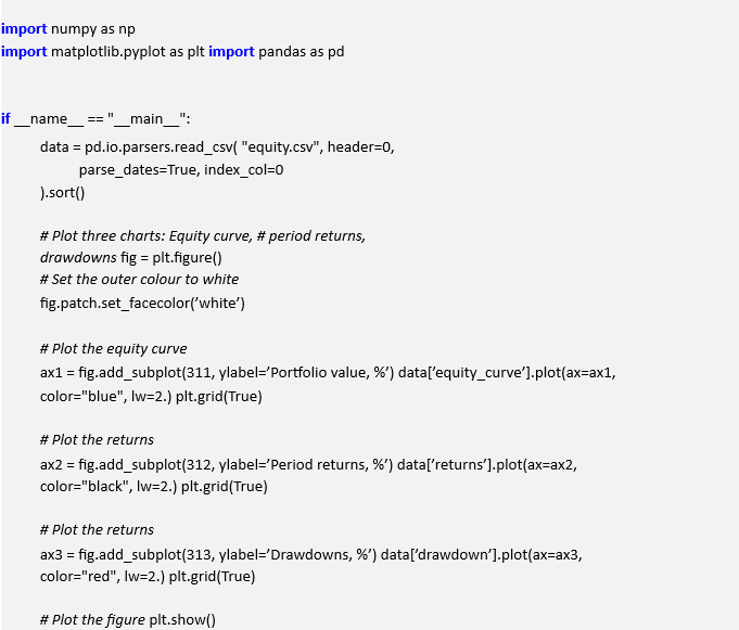
The three Figures displayed above are all created using the plot^_performance.py script. For completeness I’ve included the code so that you can use it as a base to create your own performance charts.

It is necessary to run this in the same directory as the output file from the backtest, namely where equity.csv resides. The listing is as follows: