Forecasting Algorithms In Trading

Forecasting Algorithms In Trading

In this chapter we will create a statistically robust process for forecasting financial time series. These forecasts will form the basis for further automated trading strategies. We will expand on the topic of Statistical Learning discussed in the previous chapters and use a group of classification algorithms to help us predict market direction of financial time series.

Within this chapter we will be making use of Scikit-Learn, a statistical machine learning library for Python. Scikit-learn contains “ready-made” implementations of many machine learning techniques. Not only does this save us a great deal of time in implementing our trading algorithms, but it minimises the risk of bugs introduced by our own code. It also allows additional verification against machine learning libraries written in other packages such as R or C++. This gives us a great deal of confidence if we need to create our own custom implementation, for reasons of execution speed, say.

We will begin by discussing ways of measuring forecaster performance for the particular case of machine learning techniques used. Then we will consider the predictive factors that can be used in forecasting techniques and how to choose good factors. Then we will consider various supervised classifier algorithms. Finally, we will attempt to forecast the daily direction of the S&P500, which will later form the basis of an algorithmic trading strategy.

1.) Measuring Forecasting Accuracy

Before we discuss choices of predictor and specific classification algorithms we must discuss their performance characteristics and how to evaluate them. The particular class of methods that we are interested in involves binary supervised classification. That is, we will attempt to predict whether the percentage return for a particular future day is positive or negative (i.e. whether our financial asset has risen or dropped in price).

In a production forecaster, using a regression-type technique, we would be very concerned with the magnitude of this prediction and the deviations of the prediction from the actual value.

To assess the performance of these classifiers we can make use of the following two measures, namely the Hit-Rate and Confusion Matrix.

1.1] Hit Rate:

The simplest question that we could ask of our supervised classifier is “How many times did we predict the correct direction, as a percentage of all predictions?”. This motivates the definition of the training hit rate is given by the following formula:

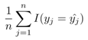
Where yˆ_j is the prediction (up or down) for the jth time period (e.g. a day) using a particular classifier. I(y_j = yˆ_j) is the indicator function and is equal to 1 if y_j = yˆ_j and 0 if y_j 6= yˆ_j.

Hence the hit rate provides a percentage value as to the number of times a classifier correctly predicted the up or down direction.

Scikit-Learn provides a method to calculate the hit rate for us as part of the classification/training process.

1.2] Confusion Matrix:

The confusion matrix (or contingency table) is the next logical step after calculating the hit rate. It is motivated by asking “How many times did we predict up correctly and how many times did we predict down correctly? Did they differ substantially?”.

For instance, it might turn out that a particular algorithm is consistently more accurate at predicting “down days”. This motivates a strategy that emphasises shorting of a financial asset to increase profitability.

A confusion matrix characterises this idea by determining the false positive rate (known statistically as a Type I error) and false negative rate (known statistically as a Type II error) for a supervised classifier. For the case of binary classification (up or down) we will have a 2×2 matrix:

Where U_T represents correctly classified up periods, U_F represents incorrectly classified up periods (i.e. classified as down), D_F represents incorrectly classified down periods (i.e. classified as up) and D_T represents correctly classified down periods.

In addition to the hit rate, Scikit-Learn provides a method to calculate the confusion matrix for us as part of the classification/training process.

2.) Factor Choice

One of the most crucial aspects of asset price forecasting is choosing the factors used as predictors. There are a staggering number of potential factors to choose and this can seem overwhelming to an individual unfamiliar with financial forecasting. However, even simple machine learning techniques will produce relatively good results when used with well-chosen factors. Note that the converse is not often the case. “Throwing an algorithm at a problem” will usually lead to poor forecasting accuracy.

Factor choice is carried out by trying to determine the fundamental drivers of asset movement. In the case of the S&P500 it is clear that the 500 constituents, in a weighted manner, will be fundamental drivers of the price, by definition! Clearly we would know the exact price of the S&P500 series if we knew the instantaneous value of its constituents, but is there any predictive power in using the prior history of returns for each constituent in predicting the series itself?

Alternatively, could we consider exchange rates with countries that carry out a lot of trade with the US as drivers of the price? We could even consider more fundamental economic and corporate factors such as interest rates, inflation, quarterly earnings.

The accuracy of the forecaster will in large part be due to the skill of the modeller in determining the right factors prior to carrying out model fitting.

2.1] Lagged Price Factors and Volume:

The first type of factor that is often considered in forecasting a time series are prior historical values of the time series itself. Thus a set of p factors could be easily obtained by creating p lags of the time series close price. Consider a daily time series. For each particular current day k, the factors would be the historical daily values at time periods k − 1, k − 2, … , k − p.

In addition to the price series itself we can also incorporate traded volume as an indicator, since it is provided when using OHLCV data (as is obtained from Yahoo Finance, Google Finance or Quandl for instance). Thus we can create a p + 1-dimensional feature vector for each day of the time series, which incorporates the p time lags and the volume series. This naturally leads to a set of pairs (X_k,y_k) representing the p + 1-dimensional feature vector X_k at day k and the actual current closing price on day k, y_k. This is all we need to begin a supervised classification exercise.

Below we will consider such a lagged time series for the S&P500 and apply multiple machine learning techniques to see if we can forecast its direction.

2.2] External Factors:

While lagged time series and volume information are a good starting point for time series analysis, we are far from restricted to such data. There are a vast amount of macroeconomic time series and asset prices series on which to consider forecasts. For instance we may wish to provide a long-term forecast of commodities prices based on weather patterns, or ascertain foreign exchange price direction movements via international interest rate movements.

If such a relationship between series can be ascertained and shown to be statistically significant, then we are at the point of being able to consider a robust trading model. We won’t dwell on such relationships too much here, as our goal is to introduce the idea of modelling and machine learning techniques. It is easy enough to form hypotheses about economic relationships and obtain the time series data either from a repository such as Quandl, or directly from government statistics websites.

3.) Classification Models

The field of machine learning is vast and there are many models to choose from, particularly in the realm of supervised classification. New models are being introduced on a monthly basis through the academic literature. It would be impractical to provide an exhaustive list of supervised classifiers in this chapter, rather we will consider some of the more popular techniques from the field.

3.1] Logistic Regression:

The first technique we will consider is logistic regression (LR). In our case we are going to use logistic regression to measures the relationship between a binary categorical dependent variable (i.e. “up” or “down” periods) and multiple independent continuous variables, such as the lagged percentage returns of a financial asset.

The logistic regression model provides the probability that a particular subsequent time period will be categorised as “up” or “down”. Thus the model introduces a parameter, namely the probability threshold for classifying whether a subsequent time period is “up” or “down”. Below, we will take this threshold to be 50% (i.e. 0.5), but it can certainly be modified to produce alternative predictions.

Logistic regression is based on the logistic formula to model the probability of obtaining an “up” day (Y = U) based on the continuous factors.

In this case, consider the situation where we are interested in predicting the subsequent time period from the previous two lagged returns, which we will denote by (L₁, L₂). The formula below gives the probability for having an up day, given that we have observed the returns on the previous time periods, L₁ and L₂:

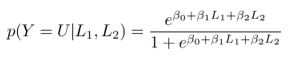
The logistic function is used instead of a linear function (i.e. in linear regression) because it provides a probability between [0,1] for all values of L₁ and L₂. In a linear regression setting it is possible to obtain negative probabilities for these continuous variables so we need another function.

To fit the model (i.e. estimate the β_i coefficients) the maximum likelihood method is used. Fortunately for us the implementation of the fitting and prediction of the logistic regression model is already handled by the Scikit-Learn library. The technique will be outlined below when we attempt to forecast the direction of the S&P500.

3.2] Discriminant Analysis:

Discriminant analysis is an alternative statistical technique to logistic regression. While logistic regression is less restrictive in its assumptions than discriminant analysis, it can give greater predictive performance if the more restrictive assumptions are met.

We will now consider a linear method and a non-linear method of discriminant analysis.

Linear Discriminant Analysis

In logistic regression we model the probability of seeing an “up” time period, given the previous two lagged returns (P(Y = U|L₁,L₂)) as a conditional distribution of the response Y given the predictors L_i, using a logistic function.

In Linear Discriminant Analysis (LDA) the distribution of the L_i variables are modelled separately, given Y , and P(Y = U|L₁,L₂) is obtained via Bayes’ Theorem.

Essentially, LDA results from assuming that predictors are drawn from a multivariate Gaussian distribution. After calculating estimates for the parameters of this distribution, the parameters can be inserted into Bayes’ Theorem in order to make predictions about which class an observation belongs to.

One important mathematical assumption of LDA is that all classes (e.g. “up” and “down”) share the same covariance matrix.

I won’t dwell on the formulae for estimating the distribution or posterior probabilities that are needed to make predictions, as once again scikit-learn handles this for us.

Quadratic Discriminant Analysis

Quadratic Discriminant Analysis (QDA) is closely reed to LDA. The significant difference is that each class can now possess its own covariance matrix.

QDA generally performs better when the decision boundaries are non-linear. LDA generally performs better when there are fewer training observations (i.e. when needing to reduce variance). QDA, on the other hand, performs well when the training set is large (i.e. variance is of less concern). The use of one or the other ultimately comes down to the bias-variance trade-off.

As with LR and LDA, Scikit-Learn takes care of the QDA implementation so we only need to provide it with training/test data for parameter estimation and prediction.

3.3] Support Vector Machines:

In order to motivate Support Vector Machines (SVM) we need to consider the idea of a classifier that separates different classes via a linear separating boundary. If such a straightforward separation existed then we could create a supervised classifier solely based on deciding whether new features lie above or below this linear classifying plane. In reality, such separations rarely exist in quantitative trading situations and as such we need to consider soft margin classifiers or Support Vector Classifiers (SVC).

SVCs work by attempting to locate a linear separation boundary in feature space that correctly classifies most, but not all, of the training observations by creating an optimal separation boundary between the two classes. Sometimes such a boundary is quite effective if the class separation is mostly linear. However, other times such separations are not possible and it is necessary to utilise other techniques.

The motivation behind the extension of a SVC is to allow non-linear decision boundaries. This is the domain of the Support Vector Machine (SVM). The major advantage of SVMs is that they allow a non-linear enlargening of the feature space to include significant non-linearity, while still retaining a significant computational efficiency, using a process known as the “kernel trick”.

SVMs allow non-linear decision boundaries via many different choices of “kernel”. In particular, instead of using a fully linear separating boundary as in the SVC, we can use quadratic polynomials, higher-order polynomials or even radial kernals to describe non-linear boundaries. This gives us a significant degree of flexibility, at the ever-present expense of bias in our estimates.

We will use the SVM below to try and partition feature space (i.e. the lagged price factors and volume) via a non-linear boundary that allows us to make reasonable predictions about whether the subsequent day will be an up move or a down move.

3.4] Decision Trees and Random Forests:

Decision trees are a supervised classification technique that utilise a tree structure to partition the feature space into recursive subsets via a “decision” at each node of the tree.

For instance one could ask if yesterday’s price was above or below a certain threshold, which immediately partitions the feature space into two subsets. For each of the two subsets one could then ask whether the volume was above or below a threshold, thus creating four separate subsets. This process continues until there is no more predictive power to be gained by partitioning.

A decision tree provides a naturally interpretable classification mechanism when compared to the more “black box” opaque approaches of the SVM or discriminant analysers and hence are a popular supervised classification technique.

As computational power has increased, a new method of attacking the problem of classification has emerged, that of ensemble learning. The basic idea is simple. Create a large quantity of classifiers from the same base model and train them all with varying parameters. Then combine the results of the prediction in an average to hopefully obtain a prediction accuracy that is greater than that brought on by any of the individual constituents.

One of the most widespread ensemble methods is that of a Random Forest, which takes multiple decision tree learners (usually tens of thousands or more) and combines the predictions. Such ensembles can often perform extremely well. Scikit-Learn handily comes with a RandomForestClassifier (RFC) class in its ensemble module.

The two main parameters of interest for the RFC are n_estimators, which describes how many decision trees to create, and n_jobs, which describes how many processing cores to spread the calculations over. We will discuss these settings in the implementation section below.

3.5] Principal Components Analysis:

All of the above techniques outlined above belong in the supervised classification domain. An alternative approach to performing classification is to not supervise the training procedure and instead allow an algorithm to ascertain “features” on its own. Such methods are known as unsupervised learning techniques.

Common use cases for unsupervised techniques include reducing the number of dimensions of a problem to only those considered important, discovering topics among large quantities of text documents or discovering features that may provide predictive power in time series analysis.

Of interest to us in this section is the concept of dimensionality reduction, which aims to identify the most important components in a set of factors that provide the most predictability. In particular we are going to utilise an unsupervised technique known as Principal Components

Analysis (PCA) to reduce the size of the feature space prior to use in our supervised classifiers.

The basic idea of a PCA is to transform a set of possibly correlated variables (such as with time series autocorrelation) into a set of linearly uncorrelated variables known as the principal components. Such principal components are ordered according to the amount of variance they describe, in an orthogonal manner. Thus if we have a very high-dimensional feature space (10+ features), then we could reduce the feature space via PCA to perhaps 2 or 3 principal components that provide nearly all of the variability in the data, thus leading to a more robust supervised classifier model when used on this reduced dataset.

3.6] Which Forecaster?

In quantitative financial situations where there is an abundance of training data one should consider using a model such as a Support Vector Machine (SVM). However, SVMs suffer from lack of interpretibility. This is not the case with Decision Trees and Random Forest ensembles.

The latter are often used to preserve interpretability, something which “black box” classifiers such as SVM do not provide.

Ultimately when the data is so extensive (e.g. tick data) it will matter very little which classifier is ultimately used. At this stage other factors arise such as computational efficiency and scalability of the algorithm. The broad rule-of-thumb is that a doubling of training data will provide a linear increase in performance, but as the data size becomes substantial, this improvement reduces to a sublinear increase in performance.

The underlying statistical and mathematical theory for supervised classifiers is quite involved, but the basic intuition on each classifier is straightforward to understand. Also – note that each of the following classifiers will have a different set of assumptions as to when they will work best, so if you find a classifier performing poorly, it may be because the data-set being used violates one of the assumptions used to generate the theory.

Naive Bayes Classifier

While we haven’t considered a Naive Bayes Classifier in our examples above, I wanted to include a discussion on it for completeness. Naive Bayes (specifically Multinomial Naive Bayes – MNB) is good to use when a limited data set exists. This is because it is a high-bias classifier. The major assumption of the MNB classifier is that of conditional independence. Essentially this means that it is unable to discern interactions between individual features, unless they are specifically added as extra features.

For example, consider a document classification situation, which appears in financial settings when trying to carry out sentiment analysis. The MNB could learn that individual words such as “cat” and “dog” could respectively refer to documents pertaining to cats and dogs, but the phrase “cats and dogs” (British slang for raining heavily) would not be considered to be meteorological by the classifier! The remedy to this would be to treat “cats and dogs” as an extra feature, specifically, and then associate that to a meteorological category.

Logistic Regression

Logistic regression provides some advantages over a Naive Bayes model in that there is less concern about correlation among features and, by the nature of the model, there is a probabilistic interpretation to the results. This is best suited to an environment where it is necessary to use thresholds. For instance, we might wish to place a threshold of 80% (say) on an “up” or “down” result in order for it to be correctly selected, as opposed to picking the highest probability category. In the latter case, the prediction for “up” could be 51% and the prediction for “down” could be 49%. Setting the category to “up” is not a very strong prediction in this instance.

Decision Tree and Random Forests

Decision trees (DT) partition a space into a hierarchy of boolean choices that lead to a categorisation or grouping based on the the respective decisions. This makes them highly interpretable (assuming a “reasonable” number of decisions/nodes in the tree!). DT have many benefits, including the ability to handle interactions between features as well as being non-parametric.

They are also useful in cases where it is not straightforward (or impossible) to linearly separate data into classes (which is a condition required of support vector machines). The disadvantage of using individual decision trees is that they are prone to overfitting (high variance). This problem is solved using a random forest. Random forests are actually some of the “best” classifiers when used in machine learning competitions, so they should always be considered.

Support Vector Machine

Support Vector Machines (SVM), while possessing a complicated fitting procedure, are actually relatively straightforward to understand. Linear SVMs essentially try to partition a space using linear separation boundaries, into multiple distinct groups. For certain types of data this can work extremely well and leads to good predictions. However, a lot of data is not linearly-separable and so linear SVMs can perform poorly here.

The solution is to modify the kernel used by the SVM, which has the effect of allowing non-linear decision boundaries. Thus they are quite flexible models. However, the right SVM boundary needs to be chosen for the best results. SVM are especially good in text classification problems with high dimensionality. They are disadvantaged by their computational complexity, difficulty of tuning and the fact the the fitted model is difficult to interpret.

4.) Forecasting Stock Index Movement

The S&P500 is a weighted index of the 500 largest publicly traded companies by market capitalisation in the US stock market. It is often utilised as an equities benchmark. Many derivative products exist in order to allow speculation or hedging on the index. In particular, the S&P500 E-Mini Index Futures Contract is an extremely liquid means of trading the index.

In this section we are going to use a set of classifiers to predict the direction of the closing price at day k based solely on price information known at day k − 1. An upward directional move means that the closing price at k is higher than the price at k−1, while a downward move implies a closing price at k lower than at k − 1.

If we can determine the direction of movement in a manner that significantly exceeds a 50% hit rate, with low error and a good statistical significance, then we are on the road to forming a basic systematic trading strategy based on our forecasts.

4.1] Python Implementations:

For the implementation of these forecasters we will make use of NumPy, Pandas and Scikit-Learn, which were installed in the previous chapters.

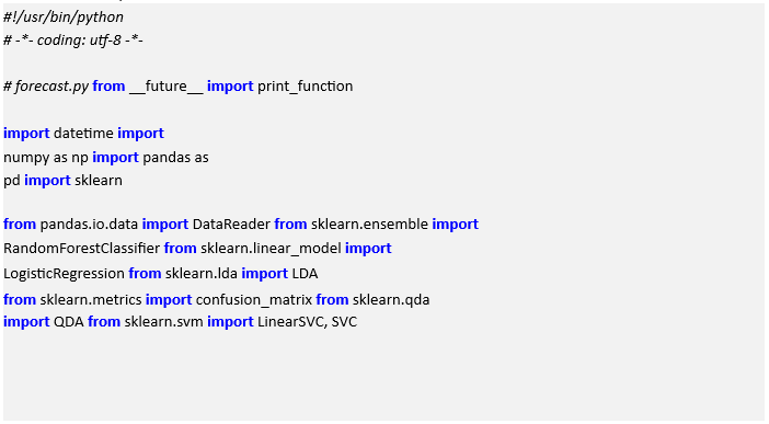
The first step is to import the relevant modules and libraries. We’re going to import the LogisticRegression, LDA, QDA, LinearSVC (a linear Support Vector Machine), SVC (a nonlinear Support Vector Machine) and RandomForest classifiers for this forecast:

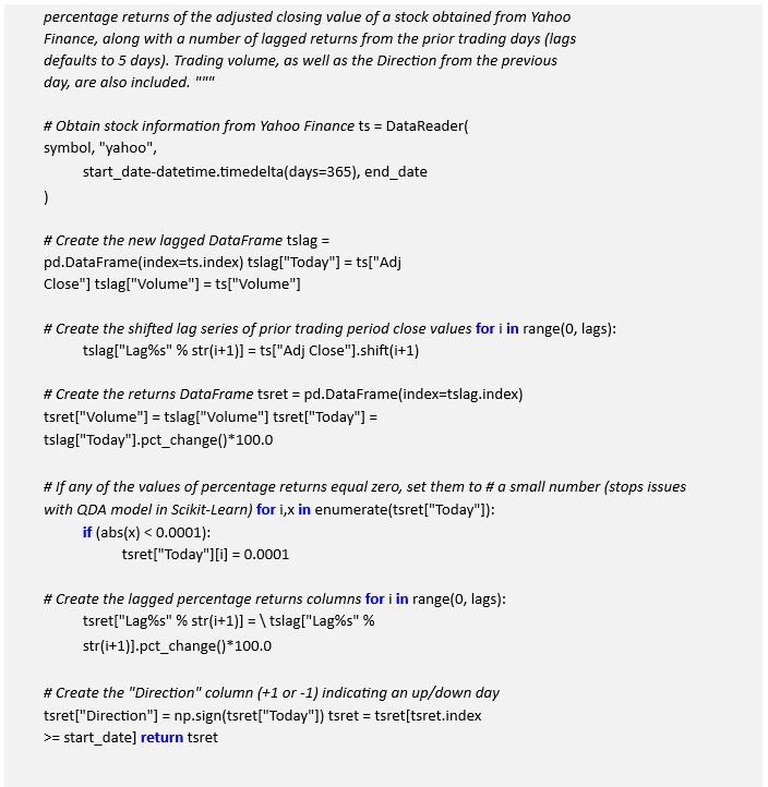
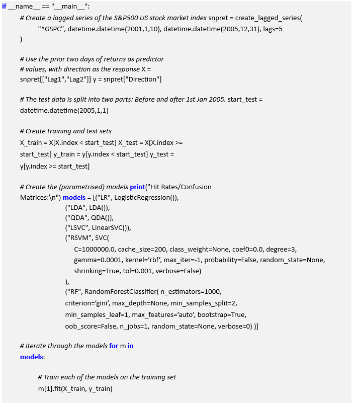
Now that the libraries are imported, we need to create a pandas DataFrame that contains the lagged percentage returns for a prior number of days (defaulting to five). create^_lagged^_series will take a stock symbol (as recognised by Yahoo Finance) and create a lagged DataFrame across the period specified. The code is well commented so it should be straightforward to see what is going on:

We tie the classification procedure together with a __main__ function. In this instance we’re going to attempt to forecast the US stock market direction in 2005, using returns data from 2001 to 2004.

Firstly we create a lagged series of the S&P500 using five lags. The series also includes trading volume. However, we are going to restrict the predictor set to use only the first two lags. Thus we are implicitly stating to the classifier that the further lags are of less predictive value. As an aside, this effect is more concretely studied under the statistical concept of autocorrelation, although this is beyond the scope of the website.

After creating the predictor array X and the response vector y, we can partition the arrays into a training and a test set. The former subset is used to actually train the classifier, while the latter is used to actually test the performance. We are going to split the training and testing set on the 1st January 2005, leaving a full trading years worth of data (approximately 250 days) for the testing set.

Once we create the training/testing split we need to create an array of classification models, each of which is in a tuple with an abbreviated name attached. While we have not set any parameters for the Logistic Regression, Linear/Quadratic Discriminant Analysers or Linear Support Vector Classifier models, we have used a set of default parameters for the Radial Support Vector Machine (RSVM) and the Random Forest (RF).

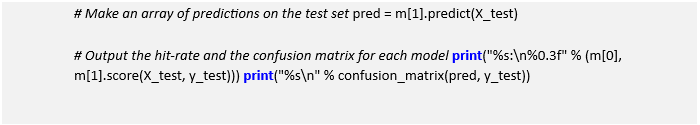
Finally we iterate over the models. We train (fit) each model on the training data and then make predictions on the testing set. Finally we output the hit rate and the confusion matrix for each model:

4.2] Results:

The output from all of the classification models is as follows. You will likely see different values on the RF (Random Forest) output as it is inherently stochastic in its construction:

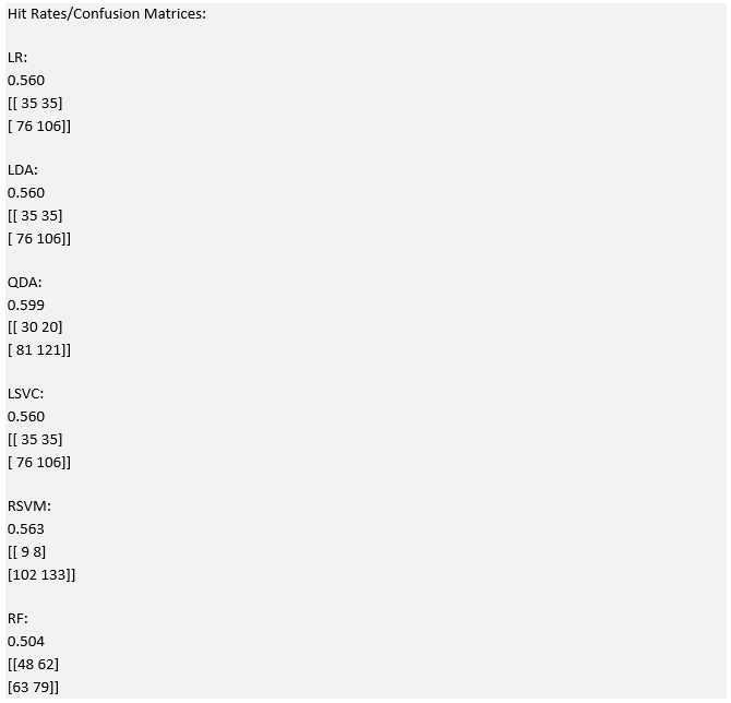
Note that all of the hit rates lie between 50% and 60%. Thus we can see that the lagged variables are not hugely indicative of future direction. However, if we look at the quadratic discriminant analyser we can see that its overall predictive performance on the test set is just under 60%.

The confusion matrix for this model (and the others in general) also states that the true positive rate for the “down” days is much higher than the “up” days. Thus if we are to create a trading strategy based off this information we could consider restricting trades to short positions of the S&P500 as a potential means of increasing profitability.

In later chapters we will use these models as a basis of a trading strategy by incorporating them directly into the event-driven backtesting framework and using a direct instrument, such as an exchange traded fund (ETF), in order to give us access to trading the S&P500.

Read Also; Time Series Analysis In Algorithmic Trading